Year 1900-1949 AD
-
1917: The coalmine Sveagruvan opens in Spitsbergen, Svalbard
-
1923: Establishment of early meteorological stations in the Soviet Arctic
-
1929: Establishment of the Unified Hydrological and Meteorological Bureau of the USSR
-
1931: Victor Franz Hess initiates measurements of cosmic rays at Hafelekar, Austria
-
1932: First navigation of the Northeast Passage without wintering
-
1933: Stalin orders the Northeast Passage made a navigable waterway
-
1939-1940: The cold winter postpones the German attack on France
-
1940: Russian icebreaker Sedow ends its drift across the Arctic Ocean
-
1940: Long sailing season and occasionally no winter ice on fjords in western Spitsbergen
-
1940: German Hilfskreuzer Komet navigates the Northeast Passage en route to the Pacific Ocean
-
1940: The Northeast Passage reported ice free from late August to late September
-
1941: February: German battleship Bismarck stuck in Hamburg because of sea ice
-
1941: May: Circumnavigating a storm centre; Bismarck’s sortie into the North Atlantic
-
1944: Worst June storm in 40 years destroys Allied harbours in Normandy
-
1947: Retreat of outletglaciers from Jostedalsbreen in southern Norway
1900:
Beginning doubts about the climatic importance of CO2

In 1900 the Swedish scientist Knut Ångström concluded that CO2 and water vapour absorb infrared radiation in the same spectral regions, thus challenging the efficacy of atmospheric CO2 as an infrared absorber. The amount of CO2 in the atmosphere was thought to be equivalent to a column of the pure gas 250 centimetres in length. Experiments done subsequently in 1905 demonstrated that a column of CO2 50 centimetres in length was sufficient for maximum absorption. Any additional CO2, it was argued, would have little or no effect on the global temperature (Fleming 1998).
Such negative assessments of CO2 were used by Charles Greely Abbot and his assistent F.E. Fowle, Jr., to insist on the primacy of water vapour as an infrared absorber in the atmosphere. This, in turn, contributed to doubts expressed by the famous geologist Thomas Chamberlin on the importance of CO2 in the atmosphere.
Click here to jump back to the list of contents.
1909-1917:
Difficult sea ice conditions around
Steamship Neptun in packice at Spitsbergen, summer 1909. Picture source: Anders Beer Wilse, Norsk Folkemuseum.
In
connection with a detailed description of the Swedish mining and exploration activities
(coal)
in
-
July 7, 1909 : The Billefjord is blocked by ice. First ship makes it to Pyramiden in innermost Billefjord July 12.
-
September 1910: Geological expedition lead by Ernest Mansfield (The Northern Exploration Co., Ltd.,
-
August 11, 1912 : Braganzavågen in Van Mijenfjorden is closed by ice. Also Bellsund is blocked by ice.
-
July 1915: An expedition lead by Birger Johnsson finds the west coast of
-
July-August 1917: Difficult sea ice conditions in Van Milenfjorden made it impossible for the steamship D/S Amsterdam to reach Braganzavågen, innermost Van Mijenfjord, before early August (see below).
Click here to see the Spitsbergen (Svalbard) meteorological series since 1912.
Click here, here and here to see later reports on sea ice conditions around Svalbard.
Click here to se Arctic sea ice data collected by DMI 1893-1961.
Click here to jump back to the list of contents.
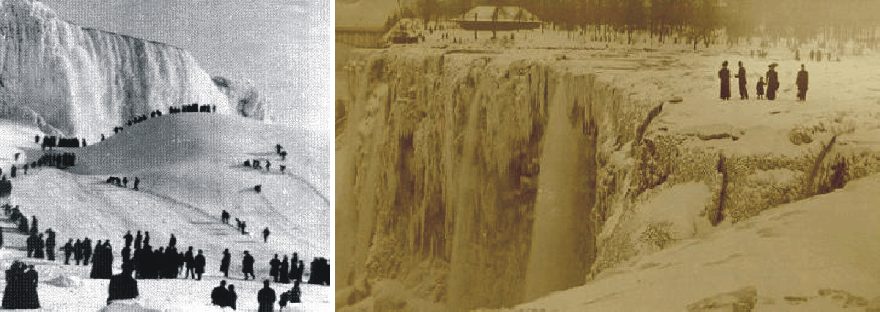
Photos showing the Niagara Falls frozen early 1911. Click here to go to the picture source.
The
winter 1910-1911 became cold in parts of North America, and resulted in surface
freezing of the Niagara Falls. People
were able to walk across from
The Niagara Falls are massive waterfalls on the Niagara River, located on the international border separating the Canadian province of Ontario and the U.S state of New York. Niagara Falls are the largest waterfall in North America. On average, about 1800 m³ water passes through the fall every second. During peak flow, the discharge may be as high as 5720 m³/s. Niagara Falls are divided into the Horseshoe Falls (792 m wide; Canada) and the American Falls (323 m wide). The height of Horseshoe Falls is about 53 m, while the height of the American Falls is lower (about 20 m), because of the presence of giant boulders at its base.
Click here to jump back to the list of contents.
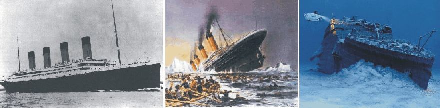
Titanic leaving Southampton 10 April 1912 (left), foundering 15 April (centre), and today sitting 3821 m below the surface of the North Atlantic (right).
Around 10:30 PM 14 April 1912 the new passenger liner Titanic on her maiden voyage to New York was steaming with about 22.5 knots across a calm sea in a clear and cold night about 400 km SE of Newfoundland. Both the air temperature and sea temperature had been dropping to a degree below freezing during the last hour. Less than 19 miles further to the west was a dense field of floating ice floes and icebergs. Almost at the same time Captain Stanley Lord, master of the freighter Californian, became thoroughly chocked as his ship with engines in full reverse rammed into this field of floating ice. Californian was lucky to escape damage, but was sitting still in the ice for the night.
At 11:40 PM an iceberg in this fatal ice field was sighted less than 900 m directly in front of Titanic. First Officer W.M. Murdoch on Titanic reacted spontaneously and in all likelihood came very close to saving the ship by a rapid port-around manoeuvre, ordering first full rudder to port and half a minute later hard to starboard, thereby swerving the liner around the iceberg in an S-shaped manoeuvre. His intention was of course to protect the all-important midship section of the hull with boilers and engines against serious damage. Presumably Murdoch actually succeeded in porting around the iceberg, but by doing this Titanic ran across an underwater extension of the iceberg and received damage to her bottom. Captain Edward J. Smith's following decision to resume steaming with reduced speed is likely to have been the actual dead sentence for the liner; the forward movement forcing large amounts of water through her damaged bottom into the hull, more than the pumps were able to cope with (Brown 2001).
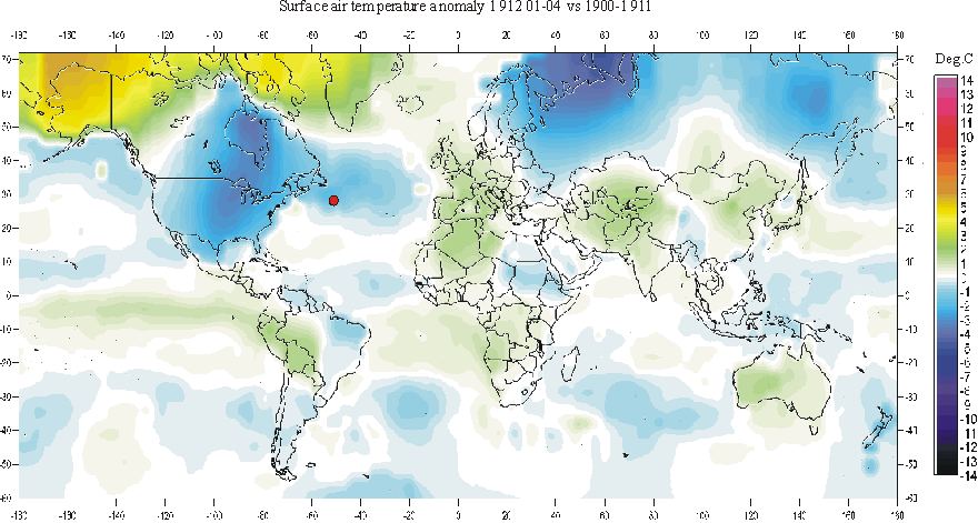
Surface air temperature anomaly January-April 1912, compared to average 1900-1911. Data source: GISS. Titanics final position SE of Newfoundland is shown by a red dot. Data source: NASA Goddard Institute for Space Studies (GISS).
Presumably
the dense field of ice floes and icebergs SE of Newfoundland came as a surprise to
Captain Smith on the fatal voyage with the Titanic. From the surface air temperature map above it
is apparent that temperature conditions January-April 1912 in this part of the
North Atlantic were several degrees below what would have been considered
‘normal’ since 1900. The warm region extending across
It is very likely that the fatal iceberg was produced by the most productive calving outlet glacier in Greenland, the Jakobshavn Isbræ.
Click here to jump back to the list of contents.
1917:
The coalmine Sveagruvan opens in Spitsbergen, Svalbard
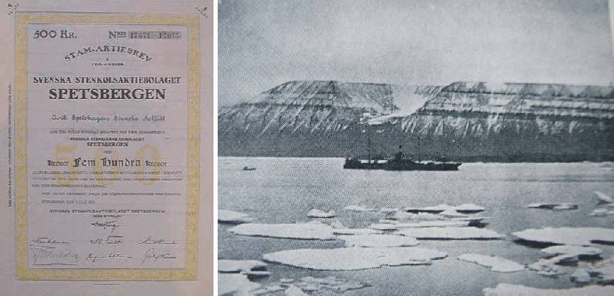
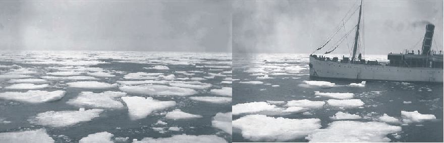
Steamship D/S Amsterdam in Braganzavågen, innermost Van Mijenfjorden, early August 1917 (right). Photo by A. Reuterskiöld.
The First World War (The Great
War; 1914-1918) resulted in a global lack of coal for energy production, and
coal prizes increased rapidly. The Swedish mining company Aktiebolaget
Spetsbergens Svenska Kolfä
The expedition left Stockholm in Sweden early July 1917 on the steamship D/S Amsterdam, but difficult sea ice conditions in Van Mijenfjorden made it impossible to reach Braganzavågen before early August (see photo above). With little doubt the summer of 1917 must have been cold compared to early 21st century conditions, as is shown by the many floes of sea ice. Today, the last floes of the winter sea ice usually melts long before August. Also the fresh snow seen in the picture is noteworthy. Snow must have been falling at low altitudes shortly before the photo was taken. The cold character of the year 1917 is clearly shown by the official Svalbard temperature record since 1912 (click here to see the entire Svalbard meteorological record), which shows all seasons of the year 1917 to be cold in comparison with previous and following years. The warming from 1917 to 1922 must indeed have been rapid in this part of the Arctic.
Under direction of Director Granholm the first buildings in the mining settlement Svea were constructed, and parts of the coming harbour for shipment of coal were established. Geological surveying was carried out in the area around the mine. About 50 persons stayed over winter along with Director Granholm, and 4,000 tonnes coal was produced, somewhat below the initial estimate of 25,000 tonnes (Hoel 1966). A layer of clay stone just above the coal layer often collapsed when the coal was removed, and it proved difficult to avoid mixing of clay stone and coal.
Click here, here and here to see other reports on sea ice conditions around Svalbard.
Click here to se Arctic sea ice data collected by DMI 1893-1961.
Click here to jump back to the list of contents.
1919-1925:
Improving sea ice conditions around
-
1919: The Swedish coal mine Sveagruvan in innermost Van Mijenfjorden is able to ship no less than 20,000 tonnes of coal, partly because of unusual fine sea ice conditions during the summer of 1919.
-
1920: The harbour at Sveagruvan is open for shipping in 98 days.
-
1921: The harbour at Sveagruvan is open for shipping in only 85 days because of difficult sea ice conditions.
-
1922: The harbour at Sveagruvan is open for shipping in 92 days. Sea ice conditions is described as ‘normal’. Report on Arctic Warming in the journal Monthly Weather Review October 10, 1922.
-
1923: The harbour at Sveagruvan is open for shipping in 97 days. Sea ice conditions is described as ‘normal’.
-
1924: The harbour at Sveagruvan is open for shipping from 9 July to 21 October (105 days). Sea ice conditions is described as ‘normal’.
-
1925: The harbour at Sveagruvan is open for shipping from 3 July to 6 October (96 days). This year the Van Mijenfjord is still free of ice when the last ship leaves October 6.
Click here to see the Spitsbergen (Svalbard) meteorological series since 1912.
Click here, here and here to see other reports on sea ice conditions around Svalbard.
Click here to se Arctic sea ice data collected by DMI 1893-1961.
Click here to jump back to the list of contents.
1922:
The changing Arctic; warming in Spitsbergen
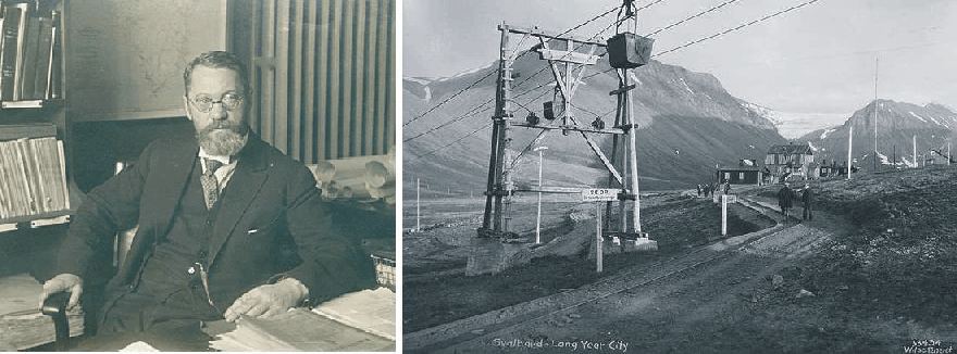
Docent Adolf Hoel in his office (left). Longyearbyen with coal mine installations around 1918 (right).
The Arctic seems to be warming up, states George Nicolas Ifft in 1922. He was at that time American consul at Bergen, Norway, and submitted from time to times reports to the the State Department, Washington, D.C. The following text represents an extract from his report, which was published in the journal Monthly Weather Review October 10, 1922.
"The Arctic seems to be warming up. Reports from fishermen, seal hunters, and explores who sail the seas about Spitsbergen and the eastern Arctic, all point to a radical change in climatic conditions, and hitherto unheard-of high temperatures in that part of the earth's surface.
In August, 1922, the Norwegian Department of Commerce sent an expedition to Spitsbergen and Bear Island under the leadership of Dr. Adolf Hoel, lecturer on geology at the University of Christiania. Its purpose was to survey and chart the lands adjacent to the Norwegian mines on those islands, take soundings of the adjacent waters, and make other oceanographic investigations.
Dr. Hoel, who has just returned, reports the location of hitherto unknown coal deposits on the eastern shores of Advent Bay - deposits of vast extent and superior quality......The oceanographic observations have, however, been even more interesting. Ice conditions were exceptional. In fact, so little ice has never before been noted. The expedition all but established a record, sailing as far north as 81o29' in ice-free water. This is the farthest north ever reached with modern oceanographic apparatus.....
In connection with Dr. Hoel's report, it is of interest to note the unusually warm summer in Arctic Norway and the observations of Capt. Martin Ingebrigtsen, who has sailed the eastern Arctic for 54 years past. He says that he first noted warmer conditions in 1918, that since that time it has steadily gotten warmer, and that to-day the Arctic of that region is not recognizable as the same region of 1868 to 1917.
Many old landmarks are so changed as to be unrecognisable. Where formerly great masses of ice were found, there are now often moraines, accumulations of earth and stones. At many points where glaciers formerly extended far into the sea they have entirely disappeared.
The change in temperature, says Captain Ingebrigtsen, has also brought about great change in the flora and fauna of the Arctic. This summer he sought for white fish in Spitsbergen waters. Formerly great shoals of them were found there. This year he saw none, although he visited all the old fishing grounds.
There were few seal in Spitzbergen waters this year, the catch being far under the average. This, however, did not surprise the captain. He pointed out that formerly the waters about Spitzbergen held an even summer temperature of about 3o Celsius; this year recorded temperatures up to 15o, and last winter the ocean did not freeze over even on the north coast of Spitsbergen.
With the disappearance of white fish and seal has come other life in these waters. This year herring in great shoals were found along the west coast of Spitsbergen, all the way from the fry to the veritable great herring. Shoals of smelt were also met with."
Click here to se Arctic sea ice data collected by DMI 1893-1961.
Click here to jump back to the list of contents.
1923:
Establishment of early meteorological stations in the Soviet Arctic
The development of Russian Arctic stations carrying out meteorological observations began around 1923 (Taracouzio 1938). The Hydrographic Office and the Arctic Institute at that time were the leading Soviet organizations interested in setting up this type of stations in the Arctic, for the conquest of the North. The function of the early stations organized by the Hydrographic Office related mainly to safety of navigation, maintaining radio communication and supplying ships with meteorological information. Those established by the Arctic Institute had scientific studies as their main purpose. The total number of stations in the Russian Arctic, however, remained small until 1929, and the quality of equipment was low (Taracouzio 1938).
Click
here to jump back to the list of contents.
1929:
Establishment of the Unified Hydrological and Meteorological Bureau of the USSR
Five
years after the first
impetus of establishing meteorological stations in the Soviet Arctic in
1923, a new period of activity began in 1929 (Taracouzio
1938). New plans for a new organization of polar stations were launched,
including additional scientific work, not always focused on navigation of the
Northern Sea Route. While the development of Soviet Arctic stations thus
received new momentum in 1929, the work of the individual stations were not done
on the basis of specific assignments relation to safety at sea, but more to
basic research.
Prior
to 1929, most geophysical work in the Soviet Arctic was limited to
meteorological observations from the few existing stations, and from ships sent
out on various expeditions. Since 1925, however, such observations had become a
more regular undertaking. It was in this year, that the Floating Weather Bureau
was organized. Two regular observers were assigned to the largest of the
icebreakers taking part of the Kara Sea expeditions, to carry out meteorological
work onboard the ships. By 1933 there were already six such floating weather
bureaus in operation on different ships navigating along the Soviet arctic coast
(Taracouzio 1938).
On 29 August 1929, the Central Executive Committee and the Council of Peoples’ Commissars of the USSR passed a joint decree, establishing the Unified Hydrological and Meteorological Bureau of the USSR. By this decree all work on meteorology, hydrology and terrestrial magnetism was concentrated in this Bureau, which shortly after (28 August) was reorganized into the Committee of the Hydrometeorological Service of the USSR. By a later decree of 11 February 1931, this Hydrometeorological Committee was transferred into the People’s Commissariat for Agriculture. Later, other existing Hydrometeorological Committtees were merged. A new decree on 23 February 1932 reorganized this Committee into the Central Administration of the Unified Hydrometeorological Service of the USSR, for short Glavsevmorput.
The high importance of Glavsevmorput is indicated by the decision of placing this organization under the direct control of the Council of People’s Commissars (Taracouzio 1938).
Click
here to jump back to the list of contents.
1930:
Birkeland draws attention to Arctic warming
One of the first scientists to publish in a scientific journal considerations on the ongoing warming in the Arctic around Svalbard was the Norwegian scientist Birkeland (1930). Apparently he was surprised to see the considerable temperature increase 1917-1923, and stated in his paper that "I would like to stress that the mean deviation results in very high figures, probably the greatest yet known on Earth".
Click here to see the Spitsbergen (Svalbard) meteorological series since 1912.
Click here to se Arctic sea ice data collected by DMI 1893-1961.
Click here to jump back to the list of contents.
1931:
Victor Franz Hess initiates measurements of cosmic rays at Hafelekar, Austria
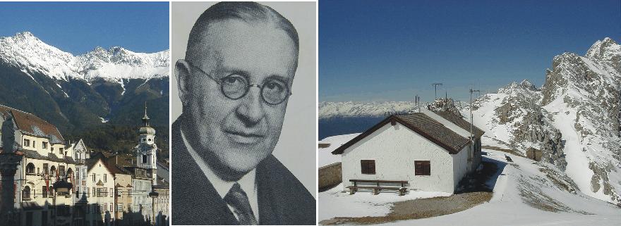
The mountain range Hafelekar seen from central Innsbruck, Austria (left). Victor Franz Hess around 1935 (centre). The still existing cosmic ray measurement station at 2300 m altitude in Hafelekar on May 21, 2000 (right).
Victor Franz Hess was born on
Victor Franz Hess was interested in radiation from radioactive material. During this work he observed a kind of radiation ("ultra radiation") which appeared to be unrelated to radioactive decay of materials in his laboratory, but had another source. He assumed that the origin of this radiation was radioactive decay of certain minerals in the bedrock below the ground surface. To investigate this hypothesis, he in 1912 carried out measurements of the "ultra radiation" from a rising balloon. To his great surprise, he found that the radiation did not decrease with altitude, but actually instead increased. This empirical falsification of his original hypothesis demonstrated that the source for this peculiar radiation was extraterrestrial, instead of being terrestrial as originally thought.
In 1919 he received the Lieben Prize for his discovery
of the "ultra-radiation" (cosmic radiation), and the year after became
Extraordinary Professor of Experimental Physics at the
In order to make more detailed
investigations of cosmic radiation possible, Hess therefore began looking for
possibilities of setting up a cosmic radiation measurement station at high
altitude. North of the city Innsbruck in western Austria a new
cableway ( the Nordkettenbahn) leading up to the Hafelekar mountains was
beginning to operate in 1928, and Hess therefore decided to make use of this
unique logistic opportunity.
The new measurement station measured
was small (4.5 x 4.5 m) and contained only one room with instruments. Later it
was enlarged with sleeping- and additional laboratory rooms (see photo above).
The central unit in the station was a cylinder filled with the gas argon.
Whenever cosmic rays penetrated the cylinder a change of the electric charge was
recorded by an electrometer, documented by automatic photography. A 1500 kg
heavy lead coating protected the argon against any other kind of radiation.
Twice a week scientists from the
Victor Franz Hess stayed at the
University of
In 1937 he returned to the
1932:
First navigation of the Northeast Passage without wintering
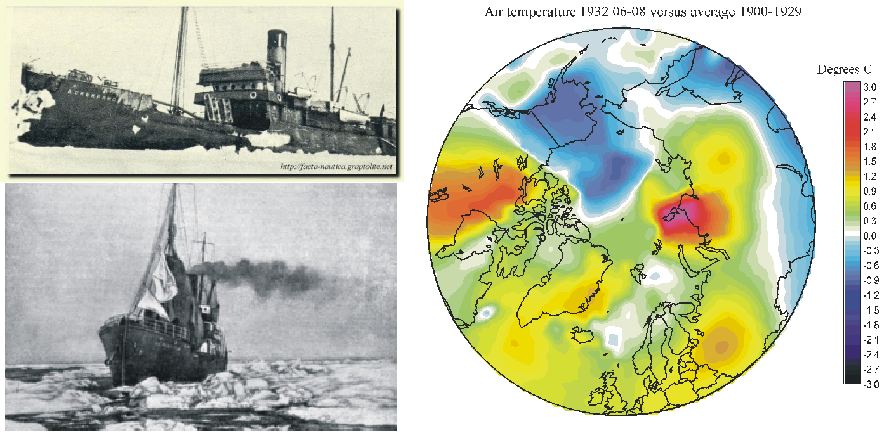
Alexandr Sibiryakov in sea ice
(left). Map showing temperatures June-August 1932, compared to the average
1900-1929 (right). The high air temperatures at the critical
point in the
Breitfuss
(1932) in the journal Polarbuch expressed pessimism in regard to the
practicability of the Northern Sea Route (The Northeast Passage).
Determined to prove the erroneousness of this the Russian Arctic Institute in
that year equipped the ship Sibiryakov for an attempt to make the passage
in one season only (Taracouzio 1938).
Sibiryakov
was was built in 1909 in
Under the command of Captain Vladimir Voronin, and with a scientific team headed by Professor Otto Smidt, Sibiryakov left Archangelsk on 28 July 1932. Having passed Matochkin Shar three days later, she reached Dickson on the western side of the large Taymyr peninsula 3 August. Exceptionally favourable ice conditions prompted Captain Voronin to enter the Laptev Sea east of the Taymyr peninsula by circumnavigating Severnaya Zemlya from the north (Taracouzio 1938), a feat very rarely repeated since, even in the early 21st century. By this Sibiryakov became the first ship to enter this part of the Arctic Ocean. Decending along the east coast of Severnaya Zemlya, however, heavy ice was encountered. Sibiryakov managed to forcing this, and arrived at Tiksi Bay east of the Lena River delta on 27 August. From there, the Chukchi Peninsula was reached without much difficulty, the sea being free from heavy ice (Taracouzio 1938). Most of the Northern Sea route was then navigated within only little more than one month. East of 167oE, however, the difficulties began. Not only had heavy ice to be forced, but the ship itself suffered damages. Its the propeller shaft broke navigating in the ice, and had to be replaced at sea. In addition Sibiryakov suffered engine troubles, and began to drift. After several days of discouraging drifting, by the use of sails, she managed to reach open water not far from the Bering Strait. On 1 October Sibiryakov entered the Bering Strait, and became the first ship to navigate the Northeast Passage in one season only.
Sibiryakov remained in service until August 1942, where she in the Kara Sea met the German pocket battle ship Admiral Scheer, and was sunk after an unequal fight.
The
impressive feat of making the first crossing without wintering was assisted by a
reduced sea ice cover following the Arctic warming following 1920. The critical
point in the passage of the
The
opening of the Northern Sea Route had the direct scientific effect, that
systematic aircraft and ship observations of sea ice from the
Click here to se Arctic sea ice data collected by DMI 1893-1961.
Click here to jump back to the
list of contents.
1933:
Stalin orders the Northeast Passage made a navigable waterway
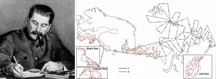
General Secretary Joseph Stalin (left). Standard airborne sea ice reconnaissance flights from 1933 (Borodachev and Shilnikov 2002). The black lines show flight paths for the air reconnaissance carried out during the season from the beginning of the programme in the last ten days of March and extending through December. The red lines show additional flight paths for the air reconnaissance carried out during the months of December, February, and March (right).
With
the Glavsevmorput
established, a decree of 17 December 1932 decided that the responsibility of all
meteorological and radio stations in the Soviet Arctic should be transferred to
this organization. To avoid administrative chaos, the existing Central
Administration of Hydrometeorology was merged with the Glavsevmorput. From 1933
the Soviet polar stations began developing into more complex bases with a wider
range of responsibilities; meteorology, radio communication, Arctic navigation
and investigations of natural resources north of 62oN (Taracouzio
1938).
Inspired
by the navigational feat of Sibiryakov
in 1932, Stalin then instructed the newly formed Glavsevmorput to make the
Northern Sea Route a navigable waterway. He clearly saw the importance of
the development of the Northeast Passage as a means in the economic
reconstruction of the USSR (Taracouzio 1938).
Results
soon became evident. The quality of technical equipment at the Soviet Arctic
stations was improved, the number of stations increased, and radio communication
was brought up to a level, where rescue work could be carried out efficiently,
should need arise.
In 1933 a total of 15 new Arctic stations were established, in 1934 no less than 26
were added to the list, and 10 new Arctic stations came into operation during
1935 (Taracouzio 1938). The Second Five-Year Plan planned 32 new stations to be
added to this list. To provide staffs qualified for the special tasks at all
these new Arctic stations, classes instituted by the Arctic Institute were
reorganized in 1933-1934 into a school where meteorologists and hydrologists
received training before commissioned to the Arctic.
A spectacular demonstration of what all this meant in practice was afforded already in 1934, when the members of the Cheliuskin expedition were rescued, after their ship was crushed and sank. It was the efficient radio communication between Moscow and the ice camp at 68o16’N, 172o51’W that enabled effective rescue to be arranged without delay.
Click here to se Arctic sea ice data collected by DMI 1893-1961.
Click here to jump back to the
list of contents.
1934:
The worst weather in the world
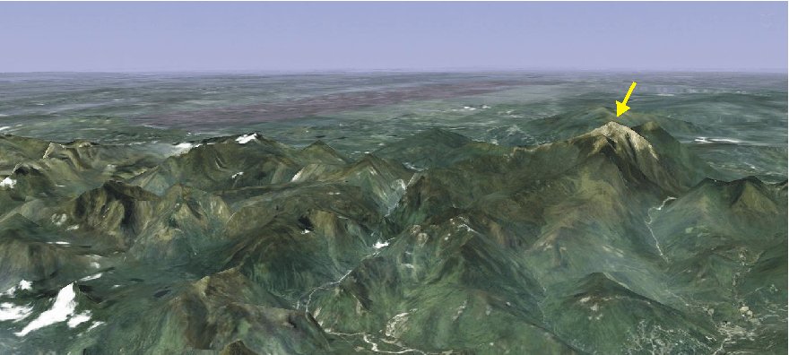
Google Earth illustration showing White Mountains in New Hampshire, USA, looking northwest. The yellow arrow indicate the summit of Mount Washington (1917 m asl).
On the summit of Mount Washington (1917 m asl), New Hampshire, USA, regular meteorological observations were conducted by the U.S. Signal Service from 1870 to 1892. The U.S. Signal Service later developed into the Weather Bureau. The Mount Washington station was the first high altitude meteorological station of its kind in the world, setting an example followed in other countries, e.g. Austria, Scotland and Norway.
The Mount Washington Observatory was reoccupied in 1932 through an impressive private initiative by a group of individuals who recognized the value of a scientific facility at such a high altitude location. In April of 1934, observers at the station measured a wind gust of 372 kilometers per hour (231 miles per hour). This still remains a world record for wind speed measured at a surface station. The station therefore proudly presents itself as the home of the world's worst weather.
Today, the Observatory continues to record and disseminate weather information. It also serves as a benchmark station for the measurement of cosmic ray activity in the upper atmosphere, and develops robust instrumentation for severe weather environments and conducts many types of severe weather research and testing. A paved road today leads to the summit and current weather conditions at the summit are available on the Internet. Since 1932, when the summit station was reoccupied, the mean annual air temperature has varied between -1.5 and -4oC, meaning that permafrost should be expected to occur near the summit even under modern climate conditions, especially in windswept sites with northerly exposure.
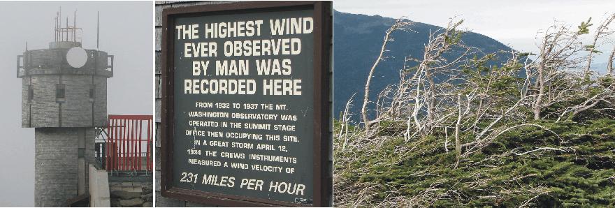
The Meteorological Observatory at the summit of Mount Washington on 13 October 2008. Notice the red metal construction protecting persons entering the station from falling rime and ice (left). Memorial plate informing about the record wind speed recorded on April 12, 1934 (centre). Windswept trees at the treeline, about 1230 m asl, looking northeast (right).
Click here to jump back to the list of contents.
1938:
Vernagtferner in Austria retreats
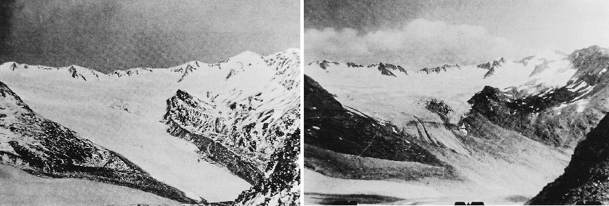
Photo showing glacier Vernagtferner in summer 1912 (left), and in July 1938 (right).
The glacier Vernagtferner continues the retreat initiated after the final large Little Ice Age advance 1844-1848. In western Austria the period 1920-1930 was relatively warm, which presumably contributed to the negative mass balance and resulting frontal retreat illustrated by comparing the two photos above. From 1912 to 1938 the glacier terminus retreated about 1200 m.
Click here, here, here and here to read about previous Little Ice Age advances of the Vernagtferner. Click here to read about the initial retreat of the glacier. Click here to read about the retreat after 1938.
Click here to jump back to the list of contents.
1939-1940:
The Finnish-USSR winter war
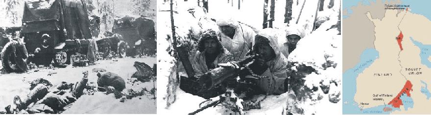
Frozen Red Army soldiers lying among deserted military vehicles in eastern Finland, December 1939 (left). Finnish machine gun team at Taipale on the Karelian front in southern Finland, January 1940 (center). Finnish areas lost to USSR by the Moscow Peace Treaty March 1940 (right).
The
Finnish-USSR Winter War began when the Soviet Union (USSR) attacked
The Red Army consequently prepared to attack Finland. The Chief of Red Army Artillery, Nikolai Voronov, just back from the rather different climate of Spain, was summoned to Kremlin. In Spain he had been a 'volunteer' under the name 'Voltaire', and his memoirs of the Spanish Civil War is perceptive and sometimes amusing. At the meeting in Kremlin October 1939 he was asked about how many days would be needed to defeat the small Finnish Army, according to his opinion. Voronov replied that he would personally be happy if everything could be resolved within two or three months. Everyone else present at the meeting laughed. The common notion was that between ten and twelve days would be sufficient (Bellamy 2007).
On
Finland
was able to mobilize an army
of 180,000 men. These troops turned out to be highly efficient with fast moving
groups of ski troops, often lead by commanders with local knowledge of the
terrain. In addition, several Finnish commanders developed a small-unit
surrounding “motti” tactics, cutting of the columns of
The
winter 1939-40 became unusually cold in
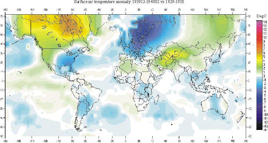
Map showing the deviation of the average surface air temperature December 1939-February 1940, compared to average conditions 1929-1938. Western Russia and Europe was exposed to very low temperatures during the winter 1939-1940, compared to the previous 10 years (1929-1938). The Finnish-USSR winter war was fought in the very centre of maximum cooling. At the same time, the winter in easternmost Siberia, Alaska and Canada was warmer than the previous 10-yr average. Data source: NASA Goddard Institute for Space Studies (GISS).
Soviet losses on the fronts
became tremendously large, and the country's international standing suffered
substantially. In the end, the general fighting ability of the Red Army was put
into question, a fact that presumably contributed to Adolf Hitler’s decision
to launch Operation
Barbarossa in June 1941.
Finland
was able to defend itself successfully until February 1940. By then,
however, it became clear that the Finnish forces were becoming exhausted, and
the Red Army had managed to penetrate the main Finnish line of defence, the
Mannerheim Line, at several places (Trotter
1991). German representatives therefore suggested that
In March 1940 the Moscow
Peace Treaty was signed, ceding about 9% of Finland's
territory and about 20% of its industrial capacity to the
At the end Voronov, the Red Army Chief of Artillery, was right: the 1939-1940 Soviet-Finnish war lasted not ten or twelve days, but instead 105 days. The Red Army's lack of preparation for fighting in the winter was partly due to the grossly optimistic estimates of how long the campaign would take, and that was a lesson well learned. The troops were ill-prepared for operations in forests and for coping with freezing weather, wrote Marchal Voronov. In addition, because of the very low temperatures, the semiautomatic mechanisms in the guns failed (Bellamy 2007). New types of lubricants had to be developed immediately. The errors made by the Red Army took time to correct, but solutions were in place a year and a half later. In December 1941 is was soldiers of the German Wehrmacht who would freeze in summer uniforms, along with their fuel and lubricants, as the Red Army moved forward in guilted jackets, fur and snow camouflage, with equipment that worked at tens of degrees Celsius below zero.
Click here to jump back to the list of contents.
1939-1940:
The cold winter postpones the German attack on France
Map showing the deviation of the average surface air temperature December 1939-February 1940, compared to average conditions 1929-1938. Both western Russia and Europe was exposed to very low temperatures during the winter 1939-1940, compared to the previous 10 years (1929-1938). At the same time, the winter in easternmost Siberia, Alaska and Canada was warmer than the previous 10-yr average. Data source: NASA Goddard Institute for Space Studies (GISS).
Immediately after the fall of the Polish capital Warsaw on 30th September 1939, Adolf Hitler ordered the German High Command to complete plans for an assault on France to the west. Speed was essential for Hitler's plans, as he was aware of Germany's lack of ability to withstand the combined industrial potential of France, the British Empire and possibly also USA, should Germany end up fighting a prolonged war.
A plan (Fall Gelb) was worked out by the Oberkommando des Heeres (OKH), with invasion of the Netherlands and Belgium, and then proceeding into northern France. The plan was superficially similar to the famous Schlieffen plan of World War I in that the main weight of the attack was to go through Belgium. The strategic aim of the plan was modest, and did not even anticipate a victory over France. It hoped just to defeat large portions of the Allied armies and gain territory in Holland.
The German 1939 attack was planned to take place on 12 November, even though several German generals were inclined to wait until the next spring. Hitler, however, remained firmly determined on launching the assault on 12 November.
Then the weather conditions intervened (Manstein 2004). The winter 1939-1940 became very cold in most of Europe (see diagram above), forcing Hitler to postpone the attack and wait for a meteorological improvement. In the new German way of conducting war, the Blitzkrieg, rapid movement of ground forces and supply columns were essential for keeping up the momentum of the attack. Poor weather and blizzards would make an unobstructed flow of much of the associated logistics difficult, and would generally be to the benefit for the defending French and British forces. In addition, the original German plans were compromised on 10 January 1940, when a staff officer of a German airborne division made a forced landing in Belgium. Before being captured, he was only partially able to burn the orders he was carrying, thereby giving away large part of the German operations plan.
At the same time the small Finnish army were putting up an astonishing defence against the much bigger Soviet Red Army further north in Europe, before ending hostilities in March 1940, and signing the Moscow Peace Treaty. The centre of cooling during the winter 1939-1940 was located precisely over the USSR-Finish battlefields, but was also clearly felt over most of Europe (see map above).
In total, Hitler had to postpone the attack no less than 15 times before the end of January 1940 (Manstein 2004), and the whole German plan of war was offset by half a year.
It is interesting to attempt an evaluation of the political significance of the cold winter 1939-1940. On one hand it gave Hitler thorough respect for military operations under winter conditions, which he later demonstrated during the planning phase of Operation Barbarossa, the German attack on USSR in June 1941. On the other hand, the Germany plan of war was offset by half a year, which was to the benefit for the Allied forces. Finally, and probably most important, the forced military interlude during the winter 1939-1940 resulted in a complete change of the German plans for the attack on France. After many heated discussions with OKH, General (later Field Marshall) Erich von Manstein's alternative plan for the campaign (Sichelschnitt) was accepted. In contrast to the original plan, this plan fully exploited the mobile and offensive capacity of the German army, with tanks negotiating the hills and narrow roads in the Ardennes. The Allies never expected a focused armoured trust across this kind of terrain. Hitler on the other hand, fully endorsed Manstein's plan.
The German attack 10 May 1940 rapidly lead to an unexpected total collapse of Allied military resistance in the Netherlands, Belgium and France. On 22 June 1940 France accepted the German terms at Compiègne, in the same railway car where the defeated Germans had signed the armistice ending World War I in 1918. On June 25 both sides ceased fire. By shifting the Schwerpunkt to the Ardennes Hitler set up the conditions for an overwhelming victory that had the potential to transform the world. This change of the operations plan may well represent the best military decision Adolf Hitler ever made (Alexander 2000). Because of the delays imposed by the cold winter 1939-1940 Germany suddenly was in a position to win the war.
Click here to jump back to the list of contents.
1940:
Russian icebreaker Sedow ends its drift across the Arctic Ocean
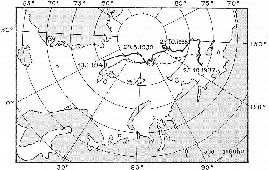
Map showing the drift of the Russian icebreaker Georgi Sedow 1937-1940 (solid line) and that of the Norwegian research vessel Fram 1893-1896 (stippled line) (Ahlmann 1941).
On January 13, 1940, the Russian icebreaker Georgi Sedow was released from the sea ice between Greenland and Svalbard, after drifting across the Arctic Ocean. This not well known event was described by the Swedish professor of Physical Geography, H.W:son Ahlman in the journal Ymer 1941, because the drift of Georgi Sedow to a high degree was nearly identical to that of the Norwegian research vessel Fram 1893-1896.
Before the 2nd World War, the Soviet Union (USSR) attempted to make use of the gradually improving summer ice conditons along the Northeast Passage, associated with the early 20th century warming. In 1932, the ship Sibiryakov was able to make the first complete navigation of the entire Northeast Passage without wintering. This interest in shipping along the Northeast Passage is the background for the establishment of a high number of meteorological stations at or near the Russian-Siberian Arctic coast in the years before the 2nd World War.
The drift of Georgi Sedow was not planned. To assist ships operating along the Northeast Passage USSR had several icebreakers stationed along the route. Even though the summer sea ice conditions were gradually improving, there was also years with more difficult ice conditions. One of these years was 1937. From time to time, the icebreakers were also used for scientific purposes. To conduct oceanographic investigations three icebreakers, Georgi Sedow, Malygin and Sadko, were stationed in the eastern part of the Laptev Sea, October 1937. Due to adverse circumstances, all tree icebreakers were beset in the ice near the starting point of the drift of Fram in 1893 (see map above), with a total crew of 217 (Ahlmann 1941).
Most of the crew (184 men) was evacuated by air in late February 1938 in an astonishing operation, leaving 33 men onboard Sadko. In June 1938 the three icebreakers Jermak, Josef Stalin and Dezjnev attempted to free the three beset ships. Josef Stalin should later assist the german auxiliary cruiser Komet during its passing of the Northeast Passage in August 1940, en route to the Pacific Ocean.
In late August 1938 Jermak actually managed to reach the beset ships on 83oN. While Malygin and Sadko now were able to steam towards ice free waters, Georgi Sedow had received serious damage to its rudder and therefore had to be towed. This, however turned out to be very difficult, and after a while it was therefore decided to leave the ship drifting with a skeleton crew of only 15 men, under the command of Captain Badygin (Ahlman 1941).
Georgi Sedow was drifting more or less parallel to the route taken by Fram 1893-1896, although following a slightly more northerly route (see map above). On January 13, 1940, the icebreaker Josef Stalin managed to reach the position of Georgi Sedow, still beset in ice, between NW Spitsbergen and Greenland (see map above). From there, Sedow was towed to Murmansk for repair.
During the drift across the Arctic Ocean, a number of scientific measurements were done by Georgi Sedow's small crew. The duration of the drift was 27 months, in contrast to the 35 month duration of the drift of Fram during the Little Ice Age. This demonstrated that the Transpolar Drift had increased in velocity, compared to the conditions experienced by Fram 1893-1896. Ahlmann (1941) notes that the velocity of this Transpolar Current apparently depends on the surface wind speed in the region. The sea water temperature was also measured by Georgi Sedow's crew, and showed significantly higher values than recorded by Fram 1893-1896 (Ahlman 1941). Also the average first year sea ice thickness was measured: it turned out to be 218 cm, compared to the 365 cm recorded by Fram about 45 years before (Ahlman 1947). Apparently, the early 20th century warming was associated with a number of significant oceanographic changes in the Arctic.
Click here to se Arctic sea ice data collected by DMI 1893-1961.
Click here to jump back to the list of contents.
1940:
Long sailing season and occasionally no winter ice on fjords in western
Spitsbergen
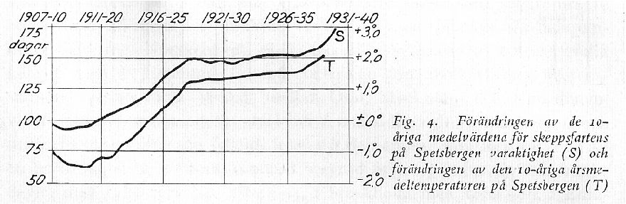
Diagram showing the change of the running 10-yr average of the length of sailing season in Spitsbergen (S) and the running 10-yr average of the mean annual air temperature in Spitsbergen (T; Ahlmann 1947).
Hesselberg and Birkeland (1940) published a paper describing the early 20th century warming in Norway and in Svalbard, finding that the mean annual air temperature in Svalbard had increased 3-4oC since 1920, mainly because of higher winter temperatures. Previously, Birkeland (1930) in a separate paper had drawn attention to the very rapid temperature increase in this part of the Arctic.
Ahlmann (1947) compares the change in air temperature with reports on the length of the sailing season to Svalbard, and produces the diagram shown above. Calculated as the average for a 10-yr period, the sailing season was at a minimum of 95 days 1909-1912, and increased to about 175 days in the period 1930-1938. In 1939 the length of the sailing season was 203 days, from 29 April to 17 November. Ahlmann (1947) himself describes the change as 'almost sensational'.
In the early part of the 20th century the sailing season to Svalbard was typically between late June and early October. Shortly before the 2nd World War, the sailing season typically began early May and ended early November, concurrent with the onset of winter darkness. This is before the invention of Radar during the 2nd World War, and few ships were eager to navigate Arctic waters in total darkness.
Ahlmann (1947) also states that during the last years leading up the the 2nd World War, little assistance from icebreakers have been required for shipping to and from Svalbard. The reason is the general reduction of sea ice around Svalbard, but also the total disappearance of winter ice on the fjords (Ahlmann 1947, p.22).
Click here, here and here to see previous reports on sea ice conditions around Svalbard.
Click here to see the Spitsbergen (Svalbard) meteorological series since 1912.
Click here to se Arctic sea ice data collected by DMI 1893-1961.
Click here to jump back to the list of contents.
1940:
German Hilfskreuzer Komet navigates the Northeast Passage en route to the
Pacific Ocean
The German auxiliary cruiser Komet,
3287 BRT (upper left). Route taken by Komet during its 516 days of operation at
sea 1940-1941, virtually taking
the ship from pole to pole (lower left). Map showing temperatures June-August
1940, compared to the average
1900-1929 (right). The high air temperatures along the
As a
tactical move against the British
naval superiority, the German navy equipped a number of Hilfskreuzers, or
auxiliary cruisers, former freighters converted into armed raiders. Keen to
establish whether a German ship could navigate the Northern Sea Route along the
Arctic coas of the Soviet Union to the Pacific, the German Naval High Command
was determined to get at least one vessel through, preferably an auxiliary
cruiser.
The
small auxiliary cruiser Komet, commanded by Kapitän zur See (later Vice Admiral)
Robert Eyssen, was asked to attempt the navigation of the Northeast Passage.
Assisted by Russian icebreaker assistance for some of the distance (see photo below),
the Komet actually managede to navigate the entire Northeast
Passage
within only two weeks, leaving Novaya Zemlya 20 August, and
reaching the Bering Strait 4 September 1940 (Barr
1975; Flaherty 2004). In 1932 Alexandr Sibiryakov
had used more than two months to complete the first navigation without
wintering.
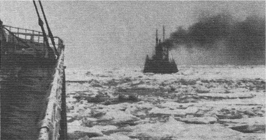
Photo taken from Komet around 26 August 1940, when the ship was following the USSR icebreaker Josef Stalin in 8/10 ice north of the Taymyr Peninsula, often one of the most difficult parts of the Northeast Passage (Eyssen 2002).
Komet was one of the smallest German II World War auxiliary cruisers. It was specially chosen by its commander Robert Eyssen because of its relatively small tonnage (3827 BRT), and the derived ability to operate in the shallow waters along the Siberian coastline. During the six months equipment time at Howaldt-Werft in Hamburg, Robert Eyssen made sure that the ships hull, rudder and propeller were enforched, to be able to operate in sea ice without danger of immediate damage (Eyssen 2002).
Apparently the Soviet Navy en route became suspicious of German intensions by sending Komet through the NE Passage, and ordered the icebreaker to leave. Presumably the Soviet government became concerned that their assistance to a German warship to reach the Pacific could be construed as a breach of their neutrality by both the UK and the USA. Komet nevertheless managed to navigate the easternmost part of the NE Passage without assistance. Robert Eyssen, however, later declared that he would not exactly be happy to repeat the experience.
Komet then
ducked down through the
Click here to se Arctic sea ice data collected by DMI 1893-1961.
Click here to jump back to the list of contents.
1940:
The Northeast Passage reported ice free from late August to late September
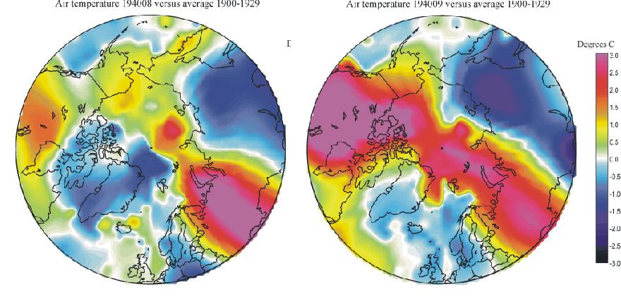
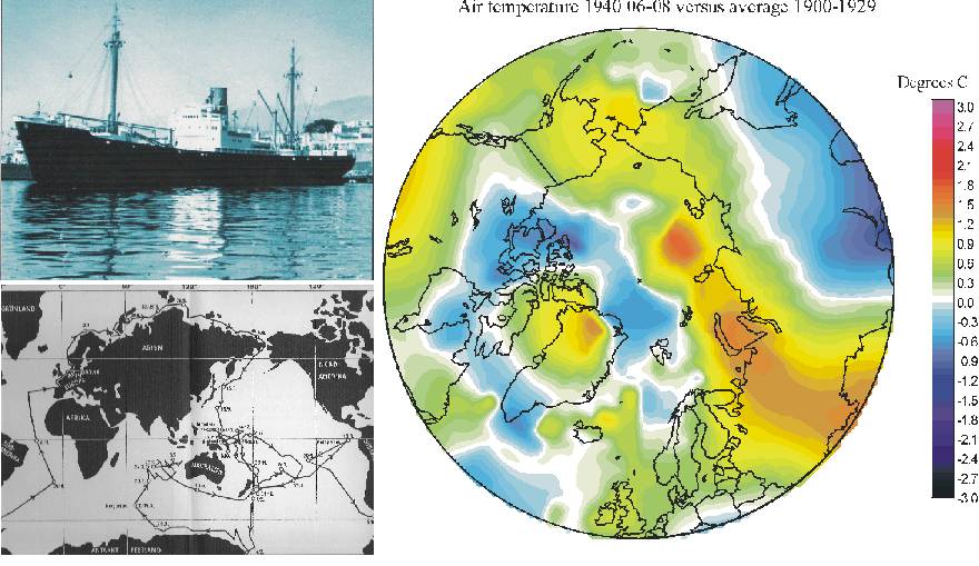
Map showing temperatures
in August (left) and September (right) 1940, compared to average conditions 1900-1929. The high air temperatures along the
Ahlmann (1947) describes changes in the Arctic sea ice cover, based on information obtained from the Arctic Institute in Leningrad, June 1945. For several years, the sea ice conditions along the arctic coast of USSR have been monitored in great detail, because of the importance for USSR shipping along the coast, and since 1939 especially because of the strategic importance of the Northeast Passage during the 2nd World War. Click here and here to see examples of military operations in these waters during the war.
According to the Arctic Institute in Leningrad ice conditions began to improve around 1920. The reduction of the summer sea ice was first recorded in the Barents Sea and in the Kara Sea to the west, and later spread to more eastern parts of the Northeast Passage. From the end of August 1940 - shortly after the passage of the German auxiliary cruiser Komet - to the end of September the entire Northeast Passage was reported free of ice (Ahlman 1947, p.305). No less than about 100 ships were operating along the USSR arctic coast during this period.
The figure above also suggest relatively warm conditions in large parts of the Arctic August-September 1940. Click here to see a another map showing how measured surface air temperatures along the USSR arctic coast indicate the presence of much open water in the summer of 1940. Click here to see a modern example of the open water effect on measured surface air temperatures in the Arctic.
Mapping of the sea ice along the USSR arctic coast from airplanes demonstrated that the summer sea ice extent from 1924 to 1944 decreased about 1 mill. km2 within the USSR part of the Arctic (Ahlmann 1947). For comparison; the reduction of Arctic summer sea ice in September 2007 (a record low value) was about 2.5 mill. km2 below the average satellite period 1979-2000 September extent for the whole Arctic Ocean.
In addition, along the route taken by the drifting Norwegian research vessel Fram across the Arctic Ocean 1893-1896, the average sea ice thickness of first year sea ice has decreased from 365 cm as recorded by Fram, to only 218 cm as recorded by the USSR icebreaker Sedow during its drift 1937-1940, roughly following the route of Fram 1893-1896 (Ahlman 1947).
Finally, Ahlmann (1947) draws attention to coastal erosion in the USSR part of the Arctic. A couple of Siberian islands consisting of ice-rich permafrost have melted completely away because of the warming, and the southern border of permafrost in Russia and Siberia has retreated towards north by several 10 km's.
Click here to se Arctic sea ice data collected by DMI 1893-1961.
Click here to jump back to the list of contents.
1941,
February: German battleship Bismarck stuck in Hamburg because of sea ice
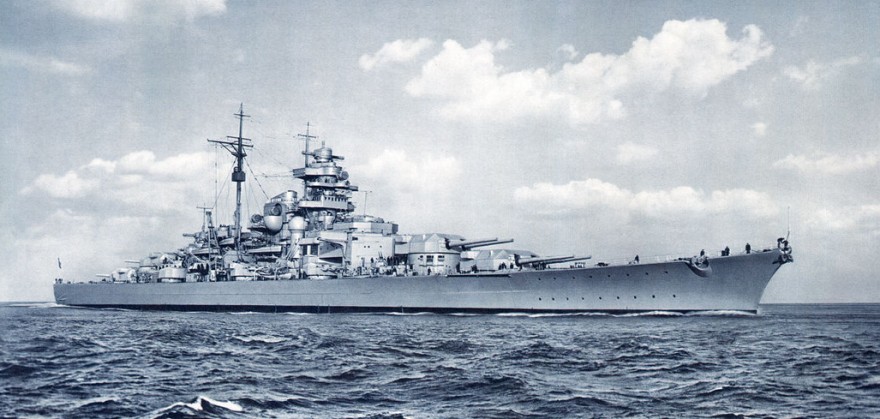
The
German battleship Bismarck
undergoing sea trials in the Baltic after raising flag in August 1940. Picture
source: www.Wehrkunst.de.
The
German battleship Bismarck and her sister-ship Tirpitz
were the largest warships to be constructed by the German Navy before and during
World War II. By the terms of the 1935 Anglo-German Naval Treaty Germany was
obliged to observe the naval treaties signed in 1922 and 1930, as well as any
treaty which might be negotiated in the future.
When
the final design of Bismarck was found to substantially exceed the 35,000 ton standard
displacement limit set by the 1936 London Treaty, several alternatives to reduce
the displacement to meet the requirements specified in the Naval Treaty were
evaluated by the German naval authorities. However, it turned out that
sufficient reductions could only be accomplished by radical design alterations;
modifying the twin main battery turret arrangement to feature either triple or
quadruple turrets, altering the main battery to a smaller calibre, changing the
split secondary battery to a dual-purpose type, or reducing the thickness and
extent of the ships armour protection (Garzke
and
Dulin 1994).
All of these changes were opposed by the German naval authorities.
It
was therefore decided to proceed with ships of 42,000 tons standard displacement
and to attempt to deceive the British and Americans regarding their real size.
The draft of these "35,000 ton" ships was therefore officially
reported to be only 7.9 m, while the full battle draft in reality exceeded 10 m.
In any event, the German naval authorities were convinced that Japan would
reject the 1936 London Naval Treaty and thereby invoke an escalator clause, to
take effect on 1 April 1937, permitting the construction of up to 45,000 ton
ships. So they decided to go ahead with the planning. American and British naval
constructors were however rightfully sceptical of the shallow draft and the
reported total displacement of the Bismarck when she was launched in February
1939. In reality, Bismarck turned out
to have a total displacement of 50,956 tons when battle ready in 1941 (Whitley
2003).
Bismarck
(and Tirpitz) featured a three-shaft
propulsion plant which was subdivided into separate engine and fire room
complexes by an arrangement of longitudinal and transverse bulkheads. The
propulsion arrangement resulted in a large beam and a large metacentric height,
as compared to that of most contemporary battleships, which resulted in high
stability with short periods of roll, providing at stable platform for
artillery, as desired by the German Navy. In addition these ships acquired a
low, elegant silhouette, and several of the German World War II warships
therefore from the distance displayed almost similar profiles, a fact that in
May 1941 would have fatal consequences for the famous British battleship Hood,
when she met Bismarck between Iceland and Greenland.
However,
fitting a centreline shaft and necessary sized propellers for the more than
150,000 metric horsepowers provided by Bismarck’s
three turbines required a much different stem form than was traditionally used
by previous German battleships in World War I. At the centreline of
Bismarck the stem had to be configured to give sufficient tip clearance to the
large centreline propeller to avoid troublesome vibration in the ship. This
resulted in a loss of underwater lateral area at the stem and a shift of the
lateral centre of effort forward, which created problems with the directional
stability of Bismarck. The need to provide sufficient clearance for the
centreline propeller also resulted in a longer than usual overhang in which the
two heavy rudders, their likewise heavy steering gear and the protective armour
for the steering gear were located (Garzke
and
Dulin 1994). This
particular design type led to problems for several World War II German cruisers
and battleships with triple-screw arrangement when they were damaged in the
stem, as they then were more prone to serious damage from the whipping phenomena
which occur whenever the extremities of a ship are subjected to
explosion-induced forces.
Otherwise,
Bismarck was an extremely
well-constructed battleship for its time. Presumably, Bismarck and other German
warships constructed up to and during World War II were among the most advanced
warships ships at their time. After the war, when inspecting the only heavy
German warship to survive World war II operational, the heavy cruiser Prinz
Eugen, the leading Royal Navy inspector, after having thoroughly
investigated the cruiser for no less than two weeks, expressed that he now had
the difficult task to explain to the Admiralty in London that the British Navy
would not be able to construct a ship as advanced as Prinz
Eugen (Schmalenbach 1998, p. 201).
Interesting, Prinz Eugen was the only
other German ship to accompany Bismarck on her dramatic first and last sortie into the North
Atlantic, in May 1941.
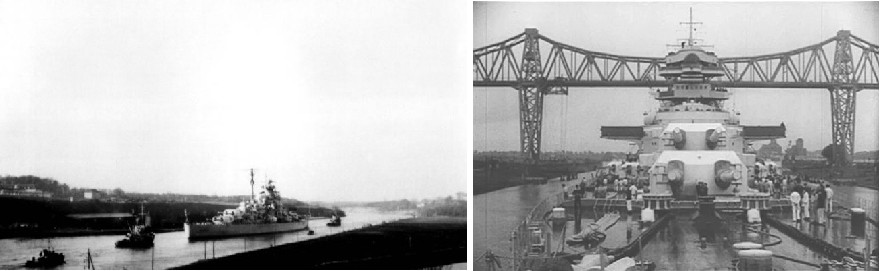
Bismarck
in the Nord-Ostsee-Kanal
(today the Kiel Canal), September 1940. The bridge seen in the picture to the
right is the
Rendsburger
Hochbrücke which was built from 1911 to 1913 and has a height of 41 meters.
Picture source: www.KBismarck.com
Bismarck
raised flag on August 24, 1940, under Captain (Kapitän zur See) Ernst
Lindemann, 45 years old and one of the navy’s ablest officers. In September
she moved from the shipyard in Hamburg to the Baltic, where the following sea
trials were supposed to take place. During these Bismarck
managed to reach a top speed of no less than 30.8 knots, thereby exceeding the
design top speed of 30.1 knots (Müllenheim-Rechberg
2005).
However,
the otherwise efficient three-propeller arrangement turned out to create serious
problems with Bismarck’s directional stability whenever the crew attempted to
steer the ship by the propellers alone, simulating a failure of both rudders.
Even with the rudders in a neutral, mid ship position, it was virtually
impossible to control the ship by the propellers alone, and eventually it always
ended up by turning into the wind. Later, in May 1941, this lack of directional
stability would turn out to have fatal consequences for Bismarck, enhanced by the meteorological situation at that time.
The
total crew of Bismarck numbered more
than 2,200, and the sea trials were supposed to take several months, perhaps
lasting until the summer of 1941. The British Royal Navy followed the progress
with keen interest, but did not expect Bismarck
to be ready for battle before June 1941 (Berthold
2005). Nevertheless, by using an efficient training scheme Captain Lindemann
hoped to have his ship ready before that.
In
early December 1940 Bismarck headed back from the Baltic to Hamburg, where the ship was
to be equipped with additional important gear at the shipyard Blohm & Voss,
the construction site of Bismarck
1937-39.
Surface
air temperature anomalies December 1940 – January 1941, compared to the
average of December-January 1929-1938. Data source: NASA Goddard
Institute for Space Studies
(GISS).
To
ensure a safe journey Bismarck was ordered to use the Nord-Ostsee-Kanal (previously
Kaiser Wilhelm-Kanal, today often called the Kiel Canal) across Schleswig-Holstein north of Hamburg, thereby avoiding the
dangerous passage of Skagerrak between Denmark and Norway, not to mention the
even more dangerous North Sea crossing to Hamburg. In both areas Bismarck would have been exposed to the might of both the British
Royal Navy and the Royal Air Force. Using the Nord-Ostsee-Kanal Bismarck
arrived safely in Hamburg on December 9, 1940. On January 24 the remaining work
on Bismarck was successfully completed, and the ship ready to return to
the Baltic for the final training of the crew, again planning to use the
Nord-Ostsee-Kanal for a safe passage. But now serious problems arose, which were
to force Captain Lindemann to abolish his plans.
Just
like the previous winter 1939-40, the winter 1940-41 turned out to be very cold
in Europe and Russia, although very mild in entire North America. The cold
winter 1939-40 had well-known significant effects on the Finnish-USSR winter
war, and it also forced the German Führer and Reichkansler Hitler to postpone
his planned attack on France in November-December 1939, until May 1940 (Manstein
2004).
These
cold winters came as a surprise for most meteorologists, as winters during the
previous 10-15 years used to be much milder, and most climate scientists
expected this warming trend to continue. This was only few years after Callendar
(1938) published his work on atmospheric CO2, thereby reviving
the CO2-temperature hypothesis originally proposed by the
electrochemist Arrhenius (1896) and in 1918
put to rest by the geologist Chamberlain (Fleming
1998).
Nevertheless,
the fact that also the winter 1940-41 turned out abnormally cold in Europe and
Russia, eventually prompted Hitler to call for a climate workshop in Germany to
evaluate the possible risk of experiencing third cold winter 1941-42 in Europe
and Russia, as he rightfully feared that this would influence negatively on his
plans for a successful, rapid war against USSR, supposed to be initiated in May
or June 1941. The German climatologists correctly pointed out that the
likelihood of having a third very cold winter in a row 1941-42 was extremely
low, as this had never been seen before during the previous observational
period.
However,
because of the intense cold, when Bismarck
on January 24, 1941, was ready for its return journey to the Baltic, the
Nord-Ostsee-Kanal was blocked by ice. And worse, a ship transporting iron ore
had recently sunk in the channel, blocking it entirely (Müllenheim-Rechberg
2005). Usually, German salvage teams would have been able to remove the
sunken ship rapidly, but the severe ice conditions made this work extremely
difficult. Captain Lindemann therefore applied for permission to take his ship
around Jutland (Denmark) instead, but the German Naval High Command estimated
the risks by this crossing to be too high, and ordered Lindemann to remain with Bismarck
in Hamburg until the Nord-Ostsee-Kanal again was clear.
On
February 5, 1941, the Nord-Ostsee-Kanal was declared open, and Bismarck
immediately prepared to leave harbour. Then the message arrived that the
Nord-Ostsee-Kanal was still blocked by ice, and in addition, it turned out that
due to the intense cold while lying inoperative in Hamburg, a number of water
tubes and conduits were frozen and damaged. Especially in the boiler rooms all
water tubes, pressure gauges and water level instruments turned out to be
destroyed by freezing when mounted near the opening of ventilators, which had
been feeding below-freezing outside air into the rooms (Whitley
2007). So Bismarck now had to
remain in Hamburg for even longer, much to Captain Lindemann’s despair. On
February 16 the frost repair works were completed, but the Nord-Ostsee-Kanal was
still blocked, as the cold weather continued.
First
on March 6, 1941, Bismarck was able to leave Hamburg, and the ship then finally
arrived safely in Kiel on March 8, delayed for almost one and a half month
because of the harsh winter conditions.
Bismarck
spend a few days in Kiel, to take on board provisions, fuel, ammunitions and two
of the battleships planned four airplanes. Then the ship proceeded east to
Gotenhafen (now Gedynia, Poland) in East Pommeren, where it would have its base
during the final sea trials. However, because of the heavy sea ice still
covering the western Baltic Sea in March 1941, and to avoid ice damage to its
propellers, Bismarck had to follow the
old warship Schlesien, which now by
the German navy was used as an icebreaker (Müllenheim-Rechberg 2005). Schlesien was not exactly a rapid ship by 1941 standards, neither
did the sea ice add to its speed, so it was first in the afternoon of March 17,
1941, that Bismarck finally arrived in
Gotenhafen.
These
different temperature-induced delays were later to have their serious effects on
the coming operations of Bismarck. Instead of being able to leave early in 1941 on its
planned North Atlantic raid ‘Rheinübung’ (Rhine Exercise), at a time where
northern nights still were long and dark, this operation had to be postponed
considerably. When ‘Rheinübung’ eventually was carried out in late May
1941, the northern nights were short and providing only little visual protection
for a ship attempting unseen to break out in the open Atlantic ocean south of
Iceland.
Click here to jump back to the list of contents.
May
1941: Circumnavigating a storm centre; Bismarck’s sortie into the North
Atlantic
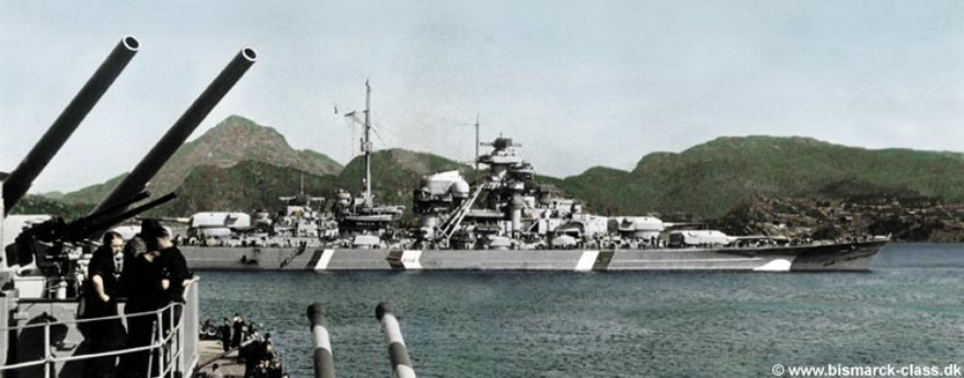
The
German battleship Bismarck near Bergen, seen from the heavy cruiser Prinz Eugen.
Probably this photo was taken in the late afternoon on 21 May 1941, shortly
before the two ships departure into the Norwegian Sea. The crew of Bismarck had
been busy the whole day by painting a new camouflage pattern (note the fake bow
wave behinds the ships real bow). The photo is taken towards E, about 2 km NE of
the present Flesland Airport. The wave pattern as well as the anchored ship’s
orientation reveals air flow from S at the time when the photo was taken.
Picture source: www.bismarck-class.dk.
After
finishing her sea trials in the Baltic in early April 1941, the German
battleship Bismarck was ready for her first sortie into the Atlantic. It was
planned that Bismarck together with the likewise new heavy cruiser Prinz
Eugen and the two small battleships Gneisenau
and Scharnhorst should form a rapid
and powerful unit. This rather formidable force would operate together during a
three-month raid in the North Atlantic, commencing in April, representing a
serious threat against British supply routes from USA and Canada. Gneisenau
and Scharnhorst had recently completed
a successful sortie into the North Atlantic under the command of Admiral Günther
Lütjens, eventually making harbour in Brest, in occupied France. It was
foreseen that Bismarck and Prinz Eugen
together should attempt breaking out into the open North Atlantic south of
Iceland via the Norwegian Sea, while Gneisenau
and Scharnhorst at the same time would
steam out from Brest. Timing was essential, as the long summer nights at
northern latitudes rapidly were approaching, making the breakout difficult.
Again Admiral Lütjens should be in command.
Then
misfortune struck. Scharnhorst had
developed metallurgical boiler problems at the end of the previous mission, and
it was now realised that the engine refit would take at least until June. Then
on April 6 Gneisenau was severely
damaged in Brest by British air raids, and was also out of action for several
months. Few days later Prinz Eugen,
just ending her final sea trials in the Baltic, was damaged by a mine near Kiel.
The whole action ‘Rheinübung’ had to be delayed until at least early May.
It
quickly was realised that neither Gneisenau
nor Scharnhorst would be able to participate in the planned raid, but
after repair Prinz Eugen would be able
to make it. Under these circumstances Admiral Lütjens preferred to postpone the
whole operation until the other new heavy German battleship, Tirpitz,
was ready in July. Grand Admiral Erich Raeder however ordered him to proceed
without delay, although the strength of his battle force now was severely
reduced; better now than later, when the USA may have entered the war and
changed the whole strategic situation. Realising how perilously the operation
would be for Bismarck and Prinz Eugen under these changed circumstances, the
commander of Tirpitz, Kapitän zur See
Karl Topp, several times asked the naval high command for permission to let his
new battleship join the battle force, even though Tirpitz’s sea trials were not yet fully completed, but in vain.
The
repair work on Prinz Eugen caused some
additional delay, but, finally, late 18 May 1941 Bismarck
and Prinz Eugen sortied separately
from Gotenhafen (now Gydnia, Poland). They were joined on 19 May by a
minesweeping flotilla and three destroyers, which would accompany them to
Norway.
While sailing through Danish waters 19-20 May on Bismarck Captain Lindemann was confronted with the geomorphological results of recurrent natural climate variations 18-19,000 years ago. Remarkably, this was to have major effects on the later developments of the German naval raid.
Bathymetrical
map showing the route (dotted red) taken by Bismarck and Prinz Eugen in southern
Kattegat in May 1941. Shallow water depths are indicated by grey colour. Depths
in meters.
At
the maximum of the last glacial period (known as the Weichselian in Europe)
about 22-23,000 years ago, the Scandinavian Ice Sheet advanced across the
present Kattegat Sea between Sweden and Denmark, to reach a maximum position
about halfway across Jutland, the main western part of Denmark. During the
following retreat towards NE, natural climatic variations from time to time made
the ice sheet readvance, producing a number of marked terminal moraines in the
Kattegat area. Several of these now submarine moraine ridges are still clearly
visible on bathymetric maps, and make navigation through Danish waters a
challenging experience for large ships, especially before the invention of GPS.
In
May 1941 Bismarck was deep in the
water, being fully supplied for a three-month raid, and without doubt the draft
of the ship exceeded 10 m. Theoretically, Bismarck might possibly have taken a route north in the western part
of Kattegat, keeping good distance to Swedish territorial waters, as the minimum
water depth for a ‘deep water’ route along the east coast of Jutland is
about 11 m. However, when a large ship enters shallow water, an airplane wing
effect occurs, but opposite, sucking the ship towards the bottom. Probably
Captain Lindemann knew that he therefore would risk hitting big boulders
protruding from the glacial sediments below, and correctly concluded that this
was not an attractive route for Bismarck, although the distance to Sweden would
make visual observations of the German flotilla impossible from there. He
therefore decided instead to take a route south and east of the Danish island
Anholt, where water depth exceeds 17 m at the most shallow point, shortly south
of Anholt.
Bismarck
and Prinz Eugen both successfully
navigated these difficult waters on 19-20 May, but this took them near Swedish
territorial waters. In the evening the German ships therefore had a short visual
encounter with the Swedish cruiser Gotland.
Without further events, the German flotilla reached a small fjord near Bergen in
western Norway around noon 21 May.
Prinz
Eugen
refuelled from a supply ship, while Bismarck did not. Prinz Eugen had a limited
cruising range of about 10,000 km (at 18 knots), while Bismack’s
range was longer, about 17,000 km (at 19 knots). Bismarck might have refuelled at Bergen, but presumably under the
impression of the developing meteorological situation, Admiral Lütjens decided
to proceed as fast as possible in the evening of 21 May, without spending time
on refuelling. In May 1941 Germany had several refuelling ships stationed at
various positions in the North Atlantic, and Bismarck could later refuel at one
of these.
One
important reason for the hasty departure from Bergen probably was that Admiral Lütjens
feared that his operation had been compromised by the chance meeting with the Gotland
in Kattegat. If so, this would reduce his chances for a passage to the North
Atlantic undetected by the British Royal Air Force and Royal Navy. In fact,
within hours after the encounter the British Admiralty in London was alerted via
sources in Sweden and ordered ships from the Home Navy to sea, including the
battlecruiser Hood and the battleship Prince
of Wales, which were ordered to take up a position south of Iceland. A
message from the German B-Dienst intelligence headquarters informed Admiral Lütjens
that at least several Royal Air Force squadrons had been alerted to the presence
of a German naval battle force in southern Norway.
Another
reason for the hasty departure was probably a Luftwaffe meteorological officer
who boarded Bismarck at Bergen, bringing the latest updated meteorological
information for the North Atlantic region. With the increasing duration of
daylight in the northern latitudes in late May, it was crucial that the weather
be sufficiently overcast to hamper British aerial and surface reconnaissance.
The Luftwaffe officer reported favourable conditions for a breakout into the
Atlantic, provided Bismarck and Prinz Eugen moved quickly. A large warm
high pressure air mass had become stagnant off the coast of the eastern United
States, a classic "Bermuda high", which sent warm air masses north
across eastern USA with cities like Washington, New York and Boston experiencing
a heat wave. In contrast, huge polar air masses were situated over
Greenland. These two air masses were colliding along a frontal zone in the
North Atlantic, causing the rapid development of a deep low pressure area with a
powerful cyclone near Iceland, associated with strong wind, severe icing
conditions and strong turbulence as high as 7 km, and snow, rain showers and
widespread fog below the clouds (Garzke and Dulin 1994). This was almost ideal
weather conditions for the planned breakout into the North Atlantic.
Thus, Admiral Lütjens had several good reasons for leaving Bergen rapidly, but whatever the exact reason, the failure to top off Bismarck's fuel tanks was later to prove to be a crucial omission. Bismarck and Prinz Eugen left Bergen by 19:30 on 21 May 1941, heading first N and later NW into the Norwegian Sea. Because of the developing low pressure near Iceland the wind was from astern, and the weather with rain, low clouds and fog. At certain times the fog reduced the sight to only 3-400 m.
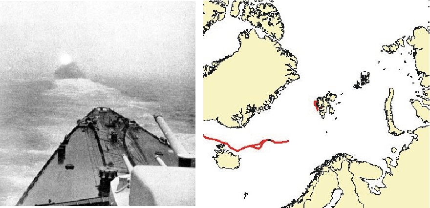
Bismarck
with search light pointed to the rear seen from Prinz Eugen during the traverse
of the Norwegian Sea on 22 May 1941 (left). Sea ice boarder between Iceland and
Greenland on 20 May 1941 (right figure; source:
http://acsys.npolar.no/ahica/quicklooks/). The existence of this unique archive
of former Arctic sea ice limits are thanks to the painstaking work of Dr. T.
Vinje at the Norwegian Polar Institute.
To
maintain formation and safe distance, the two ships had to turn on their
searchlights. By this Prinz Eugen was
able to follow closely in the wake of Bismarck at relatively high speed, about
24 knots. It was important to reach the Denmark Strait between Iceland and
Greenland, before the weather improved and the British Royal Navy was in place
to intercept. At 23:22 on 22 May Bismarck and Prinz Eugen
were north of Iceland and changed course directly to W. In the morning of 23 May
they increased speed to 27 knots and changed course toward SW, now heading for
the northern part of the Denmark Strait between Iceland and Greenland, the most
hazardous part of the attempted breakout. Simultaneously the wind turned into NE
(Müllenheim-Rechberg 2005), indicating that the German ships now were NW of the
developing storm centre.
At
15:00 on 23 May Bismarck
and Prinz Eugen ships
suddenly came out of the fog, and sailed into clear air with more than 5 km
visibility, except for scattered snow showers. Not exactly the best weather for
a breakout, but demonstrating that the two ships now had entered the cold air
masses on the NW side of the developing storm centre further south. A few
kilometres to the east, however, there was still low visibility with low clouds
and fog, and the two ships must at that time have been sailing only a few
kilometres NW of the meteorological front between the two air masses.
At
18:11 alarm was sounded on Bismarck; a ship was sighted on starboard side. A few minutes later,
however, the ship turned out to be an iceberg. The eastern limit of the arctic
sea ice along East Greenland had been reached. Usually the sea ice along East
Greenland has its maximum extension in late March or early April, so it was only
short time after the seasonal maximum. At 19:00 the limit of the dense sea ice
was reached, and the two ships now had to make frequent changes of their course
to avoid collisions with heavy ice floes while still proceeding at high speed. Prinz
Eugen was later reported to develop noise from one of its three propeller
shafts while sailing in the ice, perhaps because one of the propellers received
light damage from contact with an ice floe (Schmalenbach 1998). Further W the
summit of the Greenland Ice Sheet could be seen clearly in Bismarck’s
visual range-finding equipment (Müllenheim-Rechberg 2005).
Both
Bismarck and Prinz
Eugen were equipped with a new type of German radar, and at 19:22
indications of a ship to port were picked up. This turned out to be the heavy
British cruiser Suffolk, which recently had been equipped with a new, powerful
version of British radar, and now began following the German ships from a
position to the rear, keeping out of firing range. At 20:30 Suffolk
was joined by a second British cruiser, Norfolk. The German ships increased the
speed to more than 30 knots, and Bismarck
fired five rounds with its heavy 38 cm guns towards this new target, which
appeared on the port side to the rear. Unfortunately, the pressure blast from
the two forward main gun towers pointed obliquely astern damaged the forward
radar on Bismarck, so she now only had
the rear radar left. Admiral Lütjens therefore ordered Prinz Eugen to take up position in front of Bismarck, so the German ships still had radar capacity to probe the
ocean ahead. The British ships send a stream of position reports to London, and
to the two heavy warships Hood and Prince
of Wales, which was south of Iceland, in an excellent position to intercept
the German flotilla shortly SW of Iceland in the early morning of 24 May.
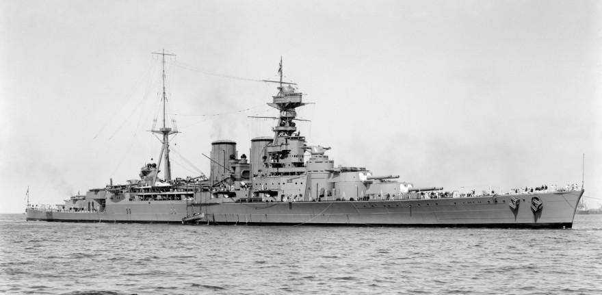
Battlecruiser
HMS Hood (47,430 tonnes).
Prince
of Wales
was a brand-new ship with a partially-trained crew and still not quite reliable
main battery turrets. Hood was
constructed in 1920, but later modernised, and in 1940 recognised as being the
pride of the British Royal British Navy. Hood was constructed to combine the
speed of a cruiser with the firepower of a battleship, and she was able to
outrun as well as outgun Bismarck. Her
main weak point was the relatively thin main deck armour, making the ship
vulnerable for steeply plunging projectiles fired over long distances. In
contrast, Bismarck was constructed to
take as well as give severe punishment at all distances, as would later be
demonstrated.
Around
5:00 on 24 May hydrophones on Prinz Eugen
picked up sounds of propellers from two fast-moving heavy vessels approaching on
the port bow. At 05:45 the German and British ships got each other in sight. The
wind was now from a northerly direction, and the German ships were still running
with the wind and waves. The still developing low pressure centre was now to the
east.
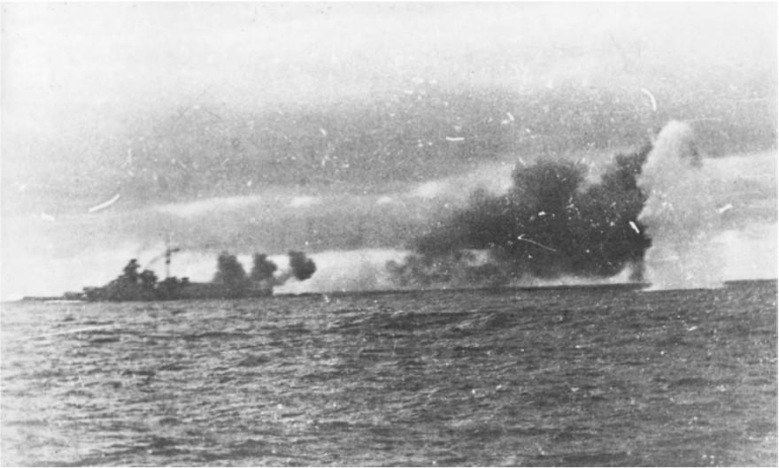
Bismarck
photographed from Prinz Eugen during the battle at Iceland, 24 May 1941. Note
the narrow and almost invisible steam trail emitted by the funnel, indicating
that turbines are driving the ship at maximum speed (30+ knots). To the right a
70 m high water impact fountain from one of Prince of Wales 35.6 cm projectiles
is seen. Bismarck’s top trained gunners are firing with 22 second intervals
(Berthold 2005), and the previous salvo cloud is seen to the right. The smoke
from the next salvo is seen just above the rear deck of Bismarck.
Bismarck is on a southerly course, and the wave pattern shows the wind to
be from N. The fact that Bismarck is able to outrun the smoke cloud shows that
the wind speed is less than 15 m/s when the photo was taken. Bismarck is 241 m
long, roughly corresponding to the distance to the previous salvo smoke cloud to
the right in the picture. So within 22 seconds Bismarck at 30+ knots was able to
outrun the tail wind with about 11 m/s, suggesting the northerly wind to be
light, about 4 m/s, as is also suggested by the wave pattern.
Hood
and Prince of Wales were commanded by
Vice Admiral Lancelot Holland, who decided to close the range to Bismarck as fast as possible, to avoid being exposed to steeply
plunging projectiles for an extended period in a long-range gunnery engagement.
At shorter range the projectiles would fly at shallow angle, where the heavy
side armour of Hood would be able to protect her efficiently. Both British ships
therefore steered directly towards Bismarck and Prinz
Eugen at full speed, even though this meant that they only were able to use
their forward guns during the approach run, while the two German ships could use
all their heavy artillery. A classical ‘crossing the T’ situation, made
famous by Admiral Horatio Nelson during the battle at Trafalgar, 21 October
1805, but at Iceland on 24 May 1941 it was the German ships that had the better
tactical position.
During
the approach run Admiral Holland ordered Hood
and Prince of Wales to fire against the leading German ship, assuming
this to be their main opponent, Bismarck.
All modern heavy German warships at that time displayed similar profile, which
obviously made Admiral Holland target the British fire on the smaller Prinz
Eugen, instead of targeting on the more dangerous Bismarck.
The Commander of Prince of Wales
however recognised the error, and rapidly turned his fire on Bismarck.
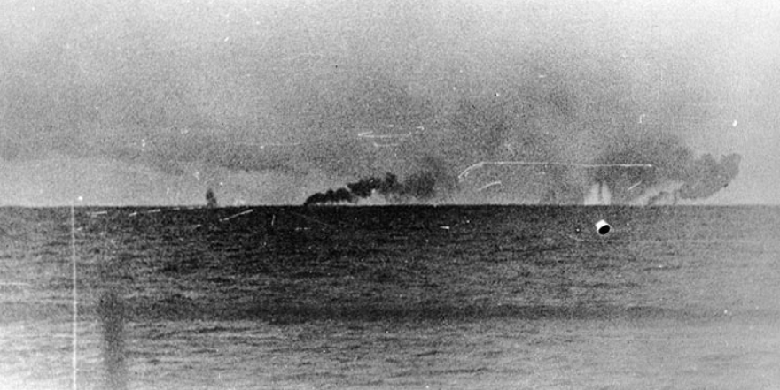
Photo
taken 24 May 1941 06:03 from Prinz Eugen, looking east. To the left the smoke
from the explosion of Hood is seen. The stern of Hood is still visible above the
water to the left of the smoke plume. To the right smoke emitted by Prince of
Wales is seen. The battleship itself is almost hidden behind water sprouts from
one of Bismarck’s salvos. The northerly wind is clearly shown by the smoke
clouds.
At
a distance of about 18 km Admiral Holland decided to turn sharply to port, to
enable all his guns to engage. However, at 05:58 while turning Hood
was hit by a salvo from Bismarck.
One or several projectiles penetrated the weak main deck armour and ignited an
ammunition magazine below. Hood
erupted in a violent explosion, breaking the mighty ship in two. Three minutes
later Hood disappeared below the surface, with only three men surviving from a
crew of 1397. Both Bismarck and Prinz
Eugen rapidly shifted their combined fire towards Prince
of Wales, who was severely hit several times, and attempted to escape in
easterly direction at full speed. Instead of giving pursuit and much to
Captain Lindemann’s dismay, Admiral Lütjens however decided to break off
the battle. He was under the general order to avoid exposing his ships to
serious danger, which might impede his later ability to operate efficiently in
the North Atlantic. As it turned out, Bismarck
had actually being hit by Prince of
Wales, seriously limiting the fuel available and causing the flooding of
one boiler room, reducing her top speed to 28 knots.
While
the battle damage on Bismarck was still being evaluated, the two German ships proceeded
in SW direction at 28 knots, still shadowed by Suffolk and Nordfolk.
Admiral Lütjens was now becoming highly impressed by the efficiency of the
new British radar. Apparently it was almost impossible to escape from
especially Suffolk, who had the more
modern equipment, bringing the entire mission in jeopardy. Admiral Lütjens
therefore planned to draw the two British cruisers across a line of seven
German submarines, waiting shortly south of Greenland, exactly with this
situation in mind (Dönitz 1997).
However,
before reaching the waiting line of submarines Admiral Lütjens realised how
seriously Bismarck’s fuel situation had become, partly due to the loss of
available fuel, partly due to the lack of refuelling while at Bergen, but also
because the British radar virtually made it virtually impossible to rendezvous
unnoticed with a German supply ship waiting near Greenland. He had no
guaranties that both pursuing British cruisers would be taken out by the
submarines. The only option left for Bismarck
apparently was to head directly for the German naval base in St.Nazaire,
France, keeping an economical speed of about 20 knots. Presumably Bismarck
was in no real danger for running out of fuel before reaching France, but this
might rapidly change, should a sea battle develop en route, where the ship had
to make use of full speed for an extended period. The course was therefore
changes from SW to SSE.
The
weather was slowly becoming windier from N with low clouds and fog, and when
entering a bank of dense fog at 03:00 in the early morning of 25 May, Bismarck
at full speed turned starboard in a wide curve, while Prinz Eugen proceeded on a southerly course, undamaged and as fast
as ever.
The
route of battleship Bismarck 18-27 May, 1942. The approximate track of the storm
centre is indicated.
Due
to the still limited range of Suffolk’s radar, both German ships actually managed to avoid being
tracked and escaped. The radarmen on Suffolk
were used to losing contact with Bismarck for
short periods as their ship zigzagged to avoid possible U-boat attacks. The fact
that Bismarck and Prinz
Eugen disappeared at 03:00 therefore initially did not alarm them very much,
but at 05:00 they had to admit that contact with the German ships had in fact
been lost permanently. At that time Bismarck
was far behind Suffolk to the north, sailing across her own wake and taking a SE
course for St. Nazaire in France. Prinz
Eugen was far ahead in the North Atlantic, where she would do what raiding
it could.
Actually,
Prinz Eugen successfully made it to
one of the German supply ships further south in the North Atlantic, but as the
fuel she received turned out to be of low quality, she soon developed serious
boiler problems and had to return to Brest in France on the 30 May (Schmalenbach
1998).
Having
lost radar contact, Suffolk for several hours navigated in a systematic search pattern,
attempting to relocate Bismarck, but
without success. On Bismarck, however,
the radar room reported receiving the radar emissions from Suffolk,
and Admiral Lütjens therefore wrongly concluded that Bismarck was still under
radar surveillance. Radar was at that time a new technical concept, and
presumably it was not realised on Bismarck
that the reflected signal was too weak to be received by Suffolk.
Lütjens in the morning of 25 May therefore decided that he could just as well
send a long radio transmission back to the German High Naval Command, explaining
details of the previous battle and Bismarck’s present fuel predicaments. This prolonged (about 30
minutes) German radio transmission quite unanticipated provided British
radio-direction finding stations with the opportunity of plotting Bismarck’s
position.
However,
a serious plotting error was made, as the initial plotting of the measured
bearing lines was done on a Mercator projection map, instead of using a gnomonic
map (displays all great circles as straight lines), which is required to plot
such lines of bearing correctly. The plotting error turned out to be quite
substantial, giving the false impression that Bismarck
was heading back towards Norway via the sea between Iceland and the Faroes. So
therefore the entire British Home Fleet steamed at full speed in a northerly
direction, while Bismarck in reality was proceeding steadily towards SE. Never
underestimate the importance of using appropriate cartography. When the
cartographic error eventually was recognised in the afternoon, Bismarck
was way ahead of all heavy British warships. In addition, because of the large
detour, several of these were beginning to run low on fuel. It looked as if Bismarck
in spite of all odds would make it safely to St. Nazaire, saved by the Mercator
map projection!
The
weather was now stormy with winds of force 9 from NW and overcast, as Bismarck
came into the air flow on the rear side of the strong storm centre now
approaching Europe. Initially this highly unpleasant weather aided Bismarck in her escape in the night to 25 May, but her course was
downwind and large following seas caused a large yaw response and significant
rolling. During trials in the Baltic, Bismarck
had demonstrated problems with directional instability due to the propeller and
rudder setup, and the combing effects of the storm, the following seas and this
slight directional instability, necessitated substantial rudder usage to
maintain the desired course towards France throughout 25 May. Presumably, the
downwind ride in the heavy sea was not too pleasant for Bismarck’s crew with its sickening, corkscrew motion.
On
the morning of 26 May the British Navy Force "H" called up from
Gibraltar was slightly north of Bismarck's
position, but without knowing it. The battlecruiser Renown,
the aircraft carrier Ark Royal and the
light cruiser Sheffield had crossed
Bismarck's track a few hours ahead of Bismarck
and were by chance close to her when a Catalina flying boat finally spotted her
at 10:30 on 26 May.
Swordfish
planes from Ark Royal then were alerted to carry out a torpedo attack on Bismarck
during the afternoon. The attack was carried out as planned, but unfortunately
it turned out that the ship being attack was not Bismarck,
but the British heavy cruise Sheffield,
which was also in the area. The error was recognized in the very last moment,
and three torpedoes already launched luckily all failed. So a new attack had to
be organized on Bismarck. But first
all airplanes had to come back to Ark
Royal, refuel and rearm and it looked as if Bismarck in the meantime was
going to disappear into the night darkness. However,
precisely at sunset
in the evening of 26 May 1941 Bismarck became
exposed to a determined torpedo attack by 15 Swordfish planes from Ark Royal.
The attack was carried out in almost unbearable weather conditions, wind force 9
from NW, low clouds and waves 8-13 m high.
Although
hampered by high waves and diminishing visibility, Captain Lindemann remarkably
at high speed outmanoeuvred most of the torpedoes coming almost synchronously
from different directions, but in the final moments of the attack Bismarck
took two torpedo hits; one of the torpedoes did not cause any serious damage,
but the final torpedo hit the rear of the ship near the two rudders. The
transient whipping response caused by this torpedo hit was stunning as the hull
acted like a springboard, and severe structural damage was sustained in the
stern structure. Possibly part of the stern settled on the rudders below,
jamming those beyond any chance of repair (Garzke and Dulin 1994).
Both
rudders jammed at a position of 12 degrees to port, as the Bismarck
was in the process of turning to evade a portside torpedo attack, and she made
two full circles before reducing speed. Once speed was reduced, the ship
unavoidably assumed a NW course into the strong wind, directly towards her
pursuers, as the intensity of the storm increased even more.
The
heavy sea and the damage done to the stern made it impossible for the damage
control teams to correct the jammed rudders, as they were unable to enter the
flooded steering compartments. Subsequent attempts to control the course of
Bismarck by the propellers failed also
because of the strong wind which forced the ship into a course against to the
wind, a weakness which already had been identified during the sea trials in the
Baltic. It has later been suggested that Bismarck
perhaps might have reached France over the stern, by sailing in aft direction
with the three undamaged propellers rotating in a special setup to compensate
for the jammed rudders. However, this would probably have been extremely
difficult – if not impossible - due to the stormy weather, and also to the
fact that all intakes for cooling water were designed with forward movement in
mind. Sailing aft over the stern for an extended period might therefore have
resulted in the turbines overheating. As is was, there was no other option than
let the turbines rotate at slow speed ahead to ensure sufficient cooling,
although this constantly brought Bismarck
closer to her pursuers. The turbines and the propellers were the only remaining
means by which Bismarck to some degree
could at least reorientate herself during the coming battle.
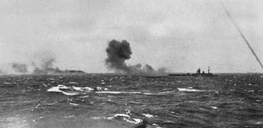
The
battleship Rodney firing at Bismarck in the morning of 27 May 1941. Bismarck is
seen in the distance, emitting smoke from fires, and slowly heading towards the
NW storm at 5-7 knots. Rodney is on an easterly course, and the smoke cloud from
the last salvo is rapidly blown ahead of the ship by the NW storm.
The
only thing which realistic might have saved Bismarck
at this point was a change of wind to easterly direction. Instead of slowly
moving towards her pursuers throughout the following night, she would then
probably have been able to make headway against the wind in easterly direction
with a speed of 15-20 knots. By this Bismarck would have been about 3-400 km
further to the east next morning, much closer to the French coast with its
potential protection by the German Luftwaffe. In addition, and perhaps more
important, she might technically have been out of reach for several of the
British warships, which during the final battle in the morning of 27 April were
dangerously low on fuel and therefore had to leave the scene before Bismarck
actually sunk. However, due to the prevailing meteorological situation, there
was no possibility for such a change in wind direction to occur in the night
between 26 and 27 May 1941. As noted by one of the survivors from Bismarck,
Baron v. Müllenheim-Rechberg (Müllenheim-Rechberg 2005), Bismarck had strangely been running with a tail wind for almost the
entire sortie into the North Atlantic, circumnavigating the storm centre.
In
the morning of 27 May 1941 Bismarck
was surrounded by a significant part of the Royal Navy. She sank at 10:39 after
being scuttled by her own crew, having lost all defensive capacity after putting
up a magnanimous fight throughout the night with several destroyers and with two
battleships since 08:47, all under completely hopeless conditions. Only 113 of
the total crew of 2065 were rescued.
The
wreck of Bismarck was discovered on 8
June 1989 by Dr. Robert D. Ballard, resting in upright position on the sediment
covered bottom of the Atlantic Ocean some 900 km west of Brest at a depth of
nearly 5 km. A large submarine landslide was released when Bismarck hit the bottom in late May 1941, today covering several
square kilometres of the ocean floor.
Click here to jump back to the list of contents.
1941: Operation Barbarossa,
the German invasion of USSR
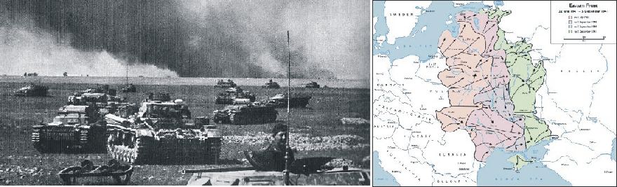
German Panzers in southern Russia July 1941 (left). Map showing the German advance until December 1941.
At
Summer, the season in which Operation Barbarossa began, was the most favourable period for military operations in European Russia. Days were long and warm, nights pleasantly cool, and only in the southern regions was the heat intense. Moors and swamps dried up, and all roads were easily passable. River discharge and water depth went down, making river crossings feasible without major problems. All arms, therefore, enjoyed optimum mobility. Even in summer, however, sudden thunderstorms could almost instantly change passable unpaved roads and open terrain into mud traps. Once the rain ended, dirt roads would dry out rapidly and could again be used by vehicles, provided that overeager drivers had not ploughed them up while still soft. During the dry periods dust often wreaked havoc on motor vehicles, clogging dust filters. But on the whole, the summer season was optimal for mobile warfare.
Spectacular German successes therefore characterized the initial phase of the Barbarossa campaign. Despite local hard Russian resistance, advances were swift. Then, from early August, the appearance of new Russian tanks superior to the German Panzers, began to slow the German advance. The German Army, even though outnumbered by the Soviet Army in soldiers, artillery and armed vehicles, still remained superior on the tactical level, and kept on pressing forward in a number of offensives. Northeast of Kiev a huge Soviet Army group 12th September were surrounded and taken prisoner in the largest encirclement achieved by either side in the entire campaign. More than 600,000 Russian soldiers were send into captivity. Nearly one third of the Soviet Army, as it had been at the outbreak of the war, was now eliminated. But notwithstanding such military successes, Adolf Hitler and the German High Command alike were taken aback by the continued strength of the Russian resistance. It became clear to them that they greatly had underestimated the number of enemy tanks and the ability of USSR to feed new divisions and new technology into the battle.
During their retreat, what they could not evacuate, the Soviet Army destroyed. Thousands of mines, steelworks and engineering plants were abandoned. Food that could not be transported was torched. By the end of 1941 the total Soviet production sank to a mere fraction of the level attained before the German invasion. The overall levels of output were never restored throughout the conflict withy Germany. The Soviet war effort, however, was sustained on the remarkable expansion of armaments and heavy-industrial output in the Urals and beyond (Overy 2006).
The victory at Kiev had encouraged many of the German General Staff to believe that one more Kesselschlact would finish the Russian Army off. October 1941, however, brought a very early onset of Winter in Russia, a few days earlier than experienced by Napoleon in 1812. On 7th October the first snow fell in western Russia. It melted rapidly, but it provoked Generaloberst Heinz Guderian to send the German Armed Forces High Command (Oberkommando der Wehrmacht; OKW) an enquiry for winter clothing. He was told that he would receive it in due course, and "not to make further unnecessary requests of this type". Guderian's army group never received any winter clothing.
Early October major German offensives were launched toward Vyazma and Bryansk 250 km southwest of Moscow. On the third day a complete break-through was accomplished, and the road to Moscow appeared wide open. Weather forecasts were, however, unfavourable and the figures for German vehicle breakdown disquietingly high. During the last three weeks of October adverse weather conditions with heavy rain, snow showers, damp and penetrating mists made movement almost impossible on two days out of three (Clark 1995).
The German army had no conception of mud as it exists in European Russia. Hitler and the OKW still believed that the mud could be conquered by brute force, an idea that lead to serious losses of vehicles and equipment. Motor vehicles broke down with clutch or engine trouble. Horses became exhausted and collapsed. Few Panzers was still operational. Large-scale operations quickly became impossible. The muddy October season 1941 probably was more severe than any other muddy season experienced during the whole German-Russian conflict in World War II (Raus 2003). Presumably the extreme mud period 10-25 October 1941 contributed as much as the following unusual cold winter to the failure of Operation Barbarossa.
A sudden frost in late October cemented one of the German 6th Panzer Division's crippled panzer columns in frozen mud, and it never again moved (Raus 2003). For the still operational units, however, the frost once again made mobile operations possible, and the German Army resumed the advance towards Moscow. Blizzards and the increasing cold, however, made the conditions for the ordinary German line divisions verging on the impossible. Many of the German soldiers were without any clothing to supplement their uniforms except denim combat overalls. The impact of the cold was intensified by the complete absence of shelter; the ground was impossible hard to dig, and most of the buildings had been destroyed in the fighting or burned by the retreating Russians. The engines of the German Panzers and other vehicles has to be run more or less continuously, in order to protect them from freezing. The state of the German fuel supplies rapidly became wretched.
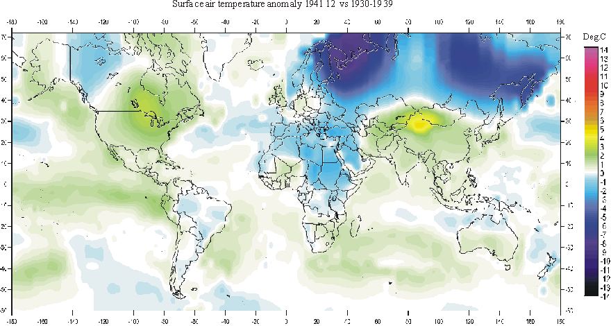
Map showing the deviation of the average surface air temperature December 1941, compared to average conditions 1930-1939. Russia and Siberia was exposed to very low temperatures, compared to the meteorological planning horizon for Operation Barbarossa (1930-1939). At the same time, UK, USA and huge areas of Canada enjoyed above average temperatures. Data source: NASA Goddard Institute for Space Studies (GISS).
Hard Russian resistance
and the cold winter finally brought Operation Barbarossa to a halt in the
vicinity of
General Raus, who was rapidly earning himself a reputation as one of the German army's foremost tacticians of armoured warfare, recorded the daily mean temperature near Moscow during the first part of December 1941 as follows (Raus 2003): 1 December -7oC, 2 December -6oC, 3 December -9oC, 4 December -36oC, 5 December -37oC, 6 December -37oC, 7 December -6oC, 8 December -8oC. Later in December temperatures again fell to no less than -45oC, and General Raus's 6th Panzer Division reported moderate and severe frostbite cases at the rate of 800 per day. The lowest temperature reported during the entire Russian campaign was -53oC, measured northwest of Moscow on 26 January (Raus 2003).
There is no reason to distrust this information on air temperatures. Contrary to common belief, German panzer divisions were not made up by panzer regiments only, but also integrated a suite of other type of units like infantry regiments, motorcycle battalions and artillery regiments. And any artillery regiment would be accompanied by meteorological units, which by balloons and other means measured temperature and wind from ground level to several kilometres altitude, to enable calculation of correct firing data. The trajectory of long-range artillery grenades would easily take them 5-6 km into the troposphere, or higher. So, in all likelihood, the information on air temperatures was measured by people with meteorological training, using proper equipment. Also Russel (1980) concludes that December 1941 was unusually cold.
The German equipment started to fail when the temperature dropped to -20oC (Ziemke 1987). At that temperature the ordinary recoil fluid used by the artillery and anti-tank weapons started to freeze, as did the lubricating oil on small arms and machine guns. This proved disastrous when the Germans had to repel ferocious counter-attacks by Russian infantry. Often only hand grenades would work. Vehicle, aircraft and even locomotive engines became extraordinary difficult to start. Tank turrets would not turn, and truck and tank engines had to be kept running constantly, which meant that a tank which did not move at all still consumed as much fuel in two days as a tank operating in battle normally did in one. In contrast, the Soviet T-34 tank, first encountered in June 1941, but only now beginning to appear in large numbers, had a compressed-air starter which could turn the engine even in the coldest weather (Bellamy 2007). In addition, its very wide tracks spread its weight so that it could roll over ditches and depressions holding 1.5 m of snow.
Just when the sudden temperature drop early December 1941 was beginning to take its toll among the German soldiers still in need of proper winter equipment, the Red Army 5 December launched a massive counterattack on the Moscow front with fresh divisions just arrived from Siberia. The Wehrmacht was pushed back from Moscow. Also the operations near Leningrad further to the northwest were severely affected by the extraordinary cold conditions. Hitler himself for the first time expressed the opinion that it perhaps would be impossible to defeat the USSR (Clark 1995). Never again would the German Wehrmacht be able to take the offensive along the entire eastern front.
It is unclear whether, as was the case with the D-Day landings in France in June 1944, Russian meteorologists were directly involved in the decision of when the Russian counteroffensive should be launched. According to German Intelligence gathered afterwards in 1942, Marshal Timoshenko had reportedly said that the Russians should go over to the attack when the first days of cold had broken the backbone of the German Army. Marshal Zhukov supposedly added that he expected the start and subsequent course of the offensive to depend on freezing off German equipment (Bellamy 2007). Russian meteorologists at that time were among the world leaders in long-range weather forecasting, and it is very likely that the Russian High Command (the Stavka) understood to make use of this meteorological knowledge. At least, from a meteorological point of view, the timing of the Russian counter-offensive at Moscow was perfect.
Click here to jump back to the list of contents.
1942:
Second ship to navigate the Northwest Passage
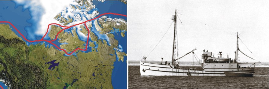
Routes through the Northwest Passage (Wikipedia; left). The Canadian RCMP (Royal Canadian Mounted Police) vessel St. Roch (right).
Built for the Royal
Canadian Mounted Police Force to serve as a supply ship for isolated, far-flung
Arctic RCMP detachments, St.
Roch (323 tons) was also designed to serve when
frozen-in for the winter as a floating detachment with its constables mounting
dog sled patrols from the ship. Between 1929 and
St
. Roch was thereby the second ship to make the passage, and the first to travel
the passage from west to east. In
Retired after returning
from the Arctic in
Click here to se Arctic sea ice data collected by DMI 1893-1961.
Click here to jump back to the list of contents.
1942:
U-435 evacuates Wettertrup "Knospe"
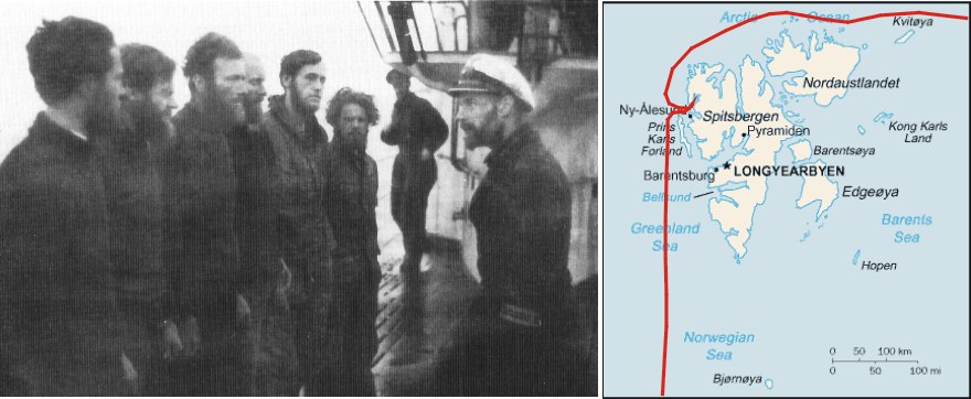
The members of the German meteorological group "Wettertrup Knospe" on the deck of German submarine U-435 on 23 August 1942, after being taken up from the shore of north-western Spitsbergen, Svalbard. The group leader H.R. Knoespel is sen to the left. The submarine commander Kapitänleutnant S. Strelow is seen to the right (left picture). Svalbard with the route taken by U-435 from south towards east (right picture).
During the II World War, Germany establisged a number of manned meteorological stations in the Atlantic sector of the Arctic, to improve weather forecasts vital for the warfare against allied convois from UK to USSR. One of the first manned stations "Knospe" was established in the inner part of Krossfjorden in northwestern Spitsbergen late 1941 under command of H.R. Knoespel, following the Norwegian and Russian populations had been evacuated in September 1941 (Selinger 2001).
It was decided to evacuate the weather station "Knospe" during the summer 1942, as the ice-free season made an allied attack possible. The submarine U-435 under the command of Kapitänleutnant S. Strelow was orderd north, to pick up the small group of 6 people from the shore. The evacuation went according to plan on 23 August 1942, without allied inteference (see photo above). The plan was to reoccupy the meteorological station again a few months later.
Instead of setting a cource directly south for the Norwegian mainland, Kapitänleutnant Strelow decided to make a detour north of Svalbard, to look for allied ships bound for Murmansk in the waters east of Svalbard and south of Franz Joseph Land (USSR). So U-435 headed north along the west coast of Spitsbergen, before turning northeast. Shortly after midnight on 26 August U-435 crossed 81oN, without ovserving ice. North of the northeastern part of Nordaustlandet was a band of ice traversed, but after that the ocean was again observed to be free of ice (Selinger 2001). U-435 finally arrived at Narvik in northern Norway on 31 August 1942.
The
ice-free
conditions observed by U-435 support similar
observations on a reduced sea ice cover in this part of the Arctic, made almost
simultaneously further east by the German heavy cruiser (pocket battleship)
Admiral
Scheer, while operating in the
Click here to se Arctic sea ice data collected by DMI 1893-1961.
Click here to jump back to the list of contents.
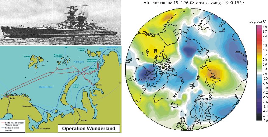
Admiral Scheer in the South Atlantic, January 1940 (above left) Map showing the route (red) taken by Admiral Scheer August 1942 (lower left). Map showing temperatures June-August 1942, compared to the average 1900-1929 (right). The high air temperatures within the operational area for Admiral Scheer most likely indicate the presence of much open water. Usually open water in the Arctic affects measured air temperatures more than the other way around. Click here to see a modern example of this open water effect recorded in Svalbard. Temperature data source: NASA Goddard Institute for Space Studies (GISS).
At 16 August
1942, the reduced sea ice along the Russian coasts of the Arctic Ocean
prompted the German Naval High Command to order the heavy cruiser (pocket battleship)
Admiral
Scheer into the
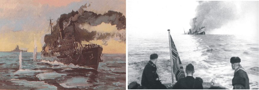
Sibiyakow under attack by Admiral Speer 25 August 1942. Photo of the sinking Sibiyakow taken by German crew member of the boat send by Admiral Sheer to evacuate the crew from Sibiryakow (Flaherty 2004).
During this so-called Operation Wunderland, Admiral Scheer, commanded by Kapitän zur See (later Vice Admiral) Wilhelm Meendsen-Bohlken, in spite of ice managed to press eastward without ice protection for the ships exposed propellers as far as 95oE. During its Arctic cruise Admiral Scheer in the Kara Sea met and promptly sank the Russian steamer Alexandr Sibiryakow (Brennecke and Krancke 2001), renowned for the first navigation of the Northern Sea Route in 1932. Admiral Scheer, however, never managed to locate any US-Canada convoy, as the Allies never attempted to make use of the NE Passage during the war.
Click
here to se Arctic sea ice data collected by DMI 1893-1961.
Click here to jump back to the list of contents.
1942:
Jakobshavn Isbræ in West Greenland retreats
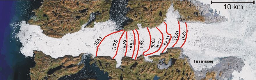
Frontal positions of calving Jakobshavn Isbræ since 1851, after reaching the maximum Little Ice Age position around 1850 (Bauer et al. 1968). Between 1893 and 1942 the glacier front retreated about 11 km. The early 21st century (2001) glacier front is seen about 4 km east of the 1942 position. According to inuit legends, the embayment Tissarissoq used to be glacier-free in the past and was used as hunting area (Hammer 1883), most likely before before the Little Ice Age glacier advance (Weidick et al. 2004). Picture source: Google Earth.
The Disko Bay region in central West Greenland (c. 70oN) is characterised by large outlet glaciers from the Greenland Ice Sheet (the Indland Ice). The major glacier Jakobshavn Isbræ is situated in a major subglacial valley, which can be traced inland for about 100 km (Echelmeyer et al. 1991). The water depth in the fjord reaches 1500 m in its outer parts (Iken et al. 1993).
Jakobshavn Isbræ is the main outlet glacier from the Greenland Ice Sheet, draining ice from about 6.5% of the total area of the ice sheet, and producing 30-45 km3 icebergs per year. This corresponds to more than 10% of the total output of icebergs from the Greenland Ice Sheet, and the Jakobshavn Isbræ is the most productive glacier in the northern hemisphere. The glacier flow velocity is also high, typically 20-22 meters per day. It is likely that the iceberg which sank Titanic in 1912 may have been produced by Jakobshavn Isbræ.
The first half of the 20th century was characterised by a 11 km frontal retreat of calving Jakobshavn Isbræ, following warming after the end of the Little Ice Age.
A more thorough description of the glacier Jakobshavn Isbræ and of the glacier retreat before 1902 can be found here. A description of the glacier retreat in the early 21st century is found here.
Click here to jump back to the list of contents.
1942-1943:
Stalingrad, a turning point of the 2nd World War
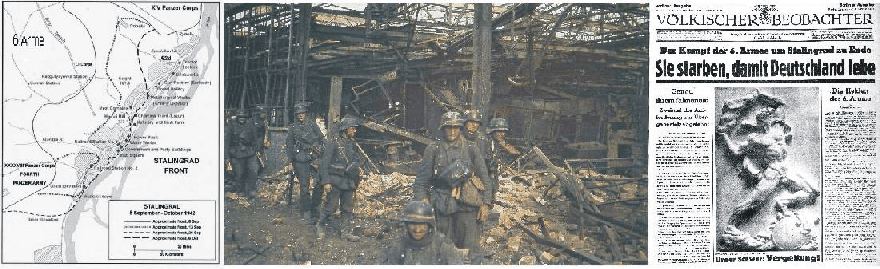
Map showing the frontline in the Stalingrad area September-October 1942 (left). German soldiers in Stalingrad October 1942 (centre). Front cover of the German newspaper Volkischer Beobachter February 4, 1943, commenting on the surrender of the 6th German Army in Stalingrad (right).
After having reorganised following the setbacks in front of Moscow during the winter 1941-1942, the German Army 28th June 1942 launched Operation Blau (Blue) in southern Russia. Three German armies split the Russian front into fragments on either side of the city Kursk, and General Hoth's eleven Panzer divisions fanned out across hundreds of miles of open rolling corn and steppe grass, towards Voronezh and the Don. Two days later also the southernmost part of the front came alive, and Field Marshal Kleist took the 1st Panzer Army across the Donetz. Soviet forces offered little resistance in the vast empty steppes and retreated eastward in disarray. By the end of July, the Wehrmacht had pushed the Red Army back across the Don River, and was standing shortly west of Stalingrad. On 19th August 1942, the 6th German Army under the command of General Friedrich Paulus reached the outskirts of Stalingrad on the western river bank of Volga, and prepared to take the city by storm.
Russian resistance around Stalingrad was organised by General Zhukov, the man who a year before had organised the frantic Russian defence of Moscow and brought the German assault there to a halt in December 1941. The responsibility of the local defence in Stalingrad was given to another very able commander, General Chuikov. The German advance into the city of Stalingrad slowed considerably down. In Stalingrad the German Army became fatally entangled in a web of street fighting, imposing on the whole army a static process of attrition which was severer than that suffered by its enemies, and to which it was less suited. By mid November, however, German Soldiers had penetrated all the way to the river bank of Volga at several places, and only small areas within Stalingrad were still held by Soviet forces.
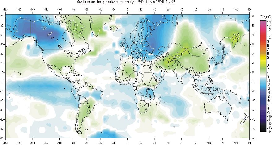
Map showing the deviation of the average surface air temperature November 1942, compared to average conditions 1930-1939. Russia and Europe was exposed to low temperatures compared to the meteorological planning horizon for the German invasion of USSR (1930-1939). Also Alaska and western Canada experienced low temperatures, while USA, eastern Canada and Greenland enjoyed above average temperatures. Data source: NASA Goddard Institute for Space Studies (GISS).
Air temperatures in Russia fell to well below average in November 1942, and most rivers froze up. Since early October General Georgy Zhukov had been planning an offensive on the southern front, with the strategic goal of by way of a pincer operation to isolate the 6th German Army in Stalingrad. The German northern flank was particularly vulnerable, since it was mainly defended by Italian, Hungarian, and Romanian units that suffered from inferior training, equipment, and morale when compared with their German counterparts. This weakness was known and exploited by the Red Army, who preferred to face off against non-German troops whenever it was possible. On the German side, the big river Don was thought to provide a safe protection for their allied troops against crossing of heavy tanks. Because of the low temperatures, however, the ice on the Don was so thick that when the Russian Operation Uranus was launched 19 November, the Russian tanks could cross the river at will. At the same time a thick frost fog covered the battlefield during the first day of the attack, heightening the general panic and confusion of the luckless Italians and Romanians. The Luftwaffe was not up to its previous strength, as substantial units 8 November were removed to counter the American landings in North Africa. Under these circumstances, the Italian and Romanian divisions did not stand a chance of bringing the Soviet offensive to a standstill.
On November 20, a second Soviet offensive was launched to the south of Stalingrad, against points held by the Romanian IV Corps. The Romanian forces, made up primarily of infantry, collapsed almost immediately. The Red Army forces raced west and northwest in a pincer movement. November 23, 1942, the tanks of the Russian 26th Armoured Corps advancing from the northwest captured the big bridge at Kalach west of Stalingrad and joined the Russian infantry that had driven up from the southeast, sealing the ring around Stalingrad. About 260,000 German military personnel were trapped in the pocket. By this they achieved something greater even than the spectacular victory which was promised by the isolation of the German 6th Army. This brilliant stroke marked the complete and final shift in the strategic balance between Soviet and Germany during the 2nd World War.
Instead of ordering an immediate
breakout and retreat from Stalingrad, Hitler ordered the 6th Army to remain at
Volga. Reichmarshal Hermann Göring assured that
the German Luftwaffe would be able to supply the besieged city from the air. The
daily needs of the 6th Army totalled about 700 tons (Alexander
2000). Though Göring's staff
apparently doubted the ability of the Luftwaffe to do anything like this after
the heavy losses sustained in the summer and autumn 1942, their chief assured
Hitler that this was entirely feasible. This
would allow the Germans in the city to fight on while a relief force was
assembled.
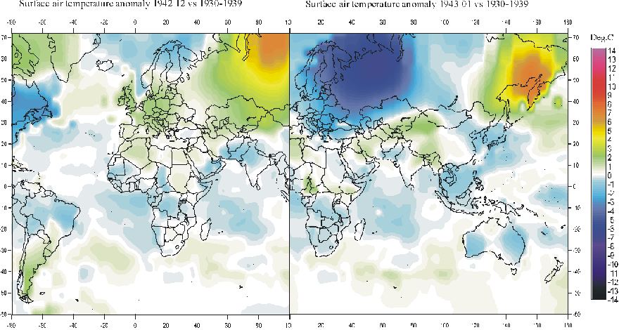
Map showing the deviation of the average surface air temperature December 1942 and January 1943, compared to average conditions 1930-1939. In December 1942 Europe, Russia and Siberia enjoyed above average temperatures. In January 1943, however, surface air temperatures in Europe and Russia decreases to well below average temperatures. Only eastern Siberia still enjoyed above average temperatures. Data source: NASA Goddard Institute for Space Studies (GISS).
The German airlift operation rapidly became a disaster. First of all, suitable airplanes for transporting the huge amount of daily supplies were only at hand in a limited number. The planned airlift operation required a force of 225 serviceable Ju 52 transports aircrafts at any time in the Stalingrad region. In fact, there was never more than 80 Junkers operational at a time (Clarck 1995). Instead, a number of Heinkel 111 bombers were ordered to participate in the supply operation. These airplanes, however, were constructed for carrying bombs, not spacious loads of food, clothing and other equipment. The transport of fuels, required special containers, which was not at hand, either.
To add to the difficulties, December 1942 in Russia turned out to be rather mild (see diagram above) due to many cyclones travelling across southern Russia. From late November appalling weather conditions spread over the whole of southern Russia with low ceiling, strong winds and snow blizzards. On one hand, the extensive cloud cover made it difficult for the Soviet air force to find and shoot down the German transport planes. On the other hand, the weather made start- and especially landing conditions almost impossible for the German airplanes. Often landings had to be cancelled because of whiteout conditions. The Heinkels, with their weaker undercarriage, often had to confine their mission to making low-level drops. Many of the Junkers broke up on landing or were destroyed by Russian artillery fire. Instead of the 550 tons promised, the air force supplied fewer than 100 ton a day, and considerably below this by the end of December and during January. The largest amount ever brought into Stalingrad in one twenty-four-hour period was 180 tons, on 14th December. After Christmas the daily average fell to about 60 tons.
Soviet forces set up a well-organised air blockade around Stalingrad, while their ground forces fought to capture the remaining German airfields. In less than two months the Luftwaffe lost 488 transport aircrafts and close to 1,000 highly experienced bomber crew personnel (Overy 2006), while German forces in Stalingrad ran short of food, ammunition and medical supplies.
German Field Marshal Erich von Manstein planned a bold overland rescue, Operation Wintergewitter. A relatively small group of German Panzer divisions gathered south of Stalingrad under the command of General Herman Hoth. On 23 December 1942 his mobile forces had managed to puch foreward to a position only 60 km from Stalingrad. At this time, however, the critical supply situation for the 6th Army made Hitler to decide against any attempt of breaking out towards Hoth's Panzer divisions. General Paulus was not the leader to disobey such orders. A renewed Soviet offensive further west made any further German rescue attempts impossible.
Almost at the same time as Operation Wintergewitter was given up, air temperatures began to fall rapidly. The Volga froze solid, allowing the Red Army to supply their forces in Stalingrad more easily. The trapped Germans rapidly ran out of heating fuel and medical supplies, and thousands started dying of frostbite, malnutrition and disease.
January 1943 became very cold (see
diagram above), with air temperatures sinking to -44oC in the
Stalingrad area. Conditions for the surrounded German soldiers rapidly
deteriorated even more. By 17 January the German occupied pocket was less than half the
original size. On 22 January the Soviet forces were able to penetrate into the
western part of the city itself, where one-third of the original German force
dug in. 30 January 1943 the bulk of the remaining German forces with just
promoted Field Marshal
Paulus surrendered. In the northern part of Stalingrad small
remaining German forces refused to accept the surrender and battled on until 2
February where they had nothing left with which to fight. According
to the German documentary film Stalingrad, over 11,000 German and Axis
soldiers refused to lay down their arms at the official surrender. These forces
continued to resist until early March 1943, hiding in cellars and sewers of the
city. By March, what remained of these forces were only small pockets of
resistance that finally surrendered.
The Battle of
Stalingrad was finally at an end, and 91,000 German soldiers became prisoners of
war. Only 5,000 survived their captivity in labor
camps and returned home. The last
handful of survivors were repatriated to Germany in 1955.
Click here to jump back to the list of contents.
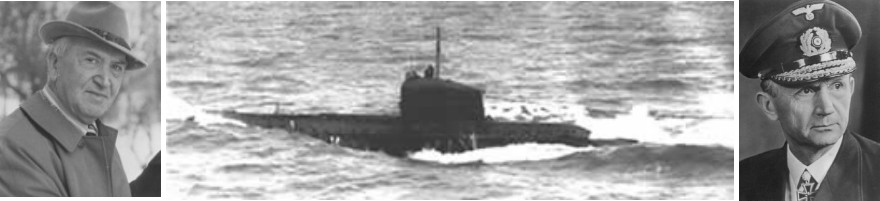
Professor Hellmuth Walter (left). Type XVII experimental Walter submarine during one of its speed trials (centre). Grand Admiral Karl Dönitz (right).
Grand
Admiral Karl Dönitz was in charge of German submarines during most of World War
II. Until 1943, the German submarine effort was, in general highly successful.
Submarines at that time had to spend a good deal of their time on the surface,
since huge quantities of air were required for the operation of their diesel
engines, which were used both for surface propulsion, and to charge the huge
batteries that were used to operate the electric motors required for submerged
propulsion. The typical German submarine type at that time had a maximum surface
speed of 15-17 knots and could only make 6-7 knots underwater. Submarines at
that time really only were a special type of surface vessels, able to dive and
operate in submerged position for some limited time.
From
1943, however, Allied advances in anti-submarine warfare, particularly the use
of airplanes flying from escort carriers, and airborne radar, made surface
operations extremely hazardous for the German submarines in the Atlantic. Within
short time, German losses of submarines increased dramatically. For that reason,
Dönitz was intensively looking for a way to remedy the situation. He therefore
turned to Professor Hellmuth Walter.
Professor
Hellmuth Walter was a brilliant engineer that in 1933 worked on a new and highly
efficient gas turbine at the Germaniawerft shipyard in Kiel. This Walter gas
turbine worked as a closed circuit propulsion system driven by hydrogen peroxide
(H2O2) in a stabilized form called Perhydrol. His ideas
were initially rejected by the Kriegsmarine in 1934 as too unconventional. In
1937, however, he managed to demonstrated his now somewhat modified design to
Kapitän zur See Karl Dönitz, who was at that time commander of a U-boat
training flotilla. Dönitz was so impressed with the proposal that he decided to
activate the proper channels in the Kriegsmarine.
In 1939 a design contract was made for a small research vessel based on
Walter’s design.
This
new type of submarine was characterized by an entirely new hydrodynamic hull
design (see photo above), making possible a surface speed of 26 knots and an
even more amazing underwater speed of 30 knots. The planned endurance of the
relatively small submarine (300 tons) was more than 4,000 km at 15 knots or
about 900 km submerged at the same speed. The experimental boat was launched on
14 April 1940, and the test results carried out were no less than sensational.
The boat reached more than 23 knots submerged which was much more than double
the maximum underwater speed of any conventional submarine in the world at that
time. In contrast to diesel engines, the Walter turbine did not rely on a supply
of fresh air. This gave the Walter submarine the ability to remain in submerged
position for extended time, which made it almost impossible to localise by
radar. This new type of submarine surely would have resulted in a revolution of submarine warfare, had a
wartime production been launched immediately. At that time, however,
Reichkansler Adolf Hitler assumed that the war would end with German victory
within short time, and no serious efforts were made to develop a military
version of the Walter submarine.
When
the German submarine crisis became a reality in 1943, Dönitz therefore ordered
the forced development and production of the still only experimental Walter
submarine. A limited number of military Walter submarines were actually produced
during the following years, but due to the advanced stage of the war none of them
managed to see enemy action. Thus the Walter boats did not have any
effect on the outcome of the war. The fuel, Perhydrol,
was highly flammable and the British Navy after the war abandoned the idea of
using the Walter turbine as too dangerous for combat vessels. Modern
submarines, however, all still make use of the efficient design of the Walter
submarine hull.
As
mentioned above, the Walter gas turbine worked as a virtually closed circuit
propulsion system, leaving only a stream of CO2 as result of the
combustion process. This CO2 had to be ventilated from the gas
turbine to the sea water outside the submarine. As described by Korvettenkapitän Peter-Erich Cremer,
it
was initially feared that the steady release of CO2 might compromise the
submarine
by leaving a track of bubbles on the sea surface. In practice, however, this turned
out not to represent a problem, as all CO2 rapidly was taken up in
solution by the surrounding sea water within a short distance of the submarine (Cremer 1988).
No compromising CO2 bubble trail was forming on the surface behind
the submerged submarine.
Click here to jump back to the list of contents.
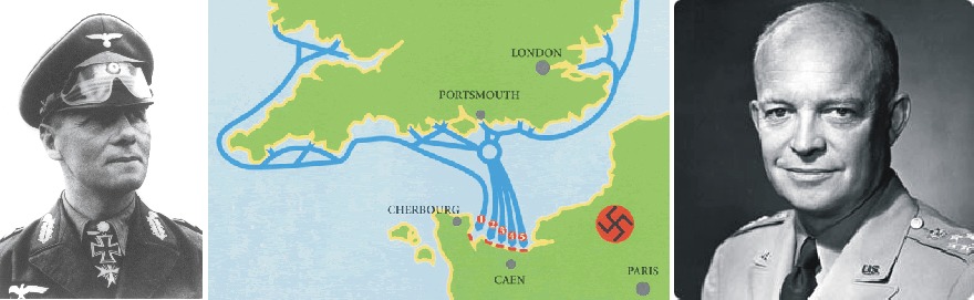
Field Marshal Erwin J.E. Rommel (left). Sea routes active during the Allied invasion of France June 6, 1944 (centre). Five-star general Dwight D. Eisenhower (right).
In 1944, two of the greatest armored commanders in history, Generaloberst
Heinz Guderian and Field Marshal Erwin Rommel, disagreed on the proper way to
meet the expected Allied invasion of
Based on his experiences in the east, Guderian recommended mobile warfare
with the German panzer and panzergrenadier diversions stationed far inland in
From
March 1944, Hitler himself actually speculated that the Allied landing might
take place in
The supreme commander of the Allied invasion forces in
On the morning of June 4, with several divisions of the invasion force
already at sea, Eisenhower and his commanders met with their
meteorological committee, headed by RAF Group Captain J.M. Stagg (Alexander
2000). Unfortunately, the weather forecast was far from being good. Low clouds, high winds,
and strong waves were forecasted for the planned invasion day, June 5.
Eisenhower had to postpone the invasion for one day. The problem was that
postponing the operation beyond June 6 or 7 would involve rescheduling the
entire invasion and creating problems of enormous magnitude.
Eisenhower's decision was, however, very wise. In the early morning of June 5, a
wind of almost hurricane force, along with sheets of rain, pondered the invasion
coast. But at the same time, due to their network of meteorological observations
from the
German meteorologists were well aware of the coming bad weather. But due
to their much more limited number of meteorological data from the
Rommel was frustrated by his lack of direct command over the panzer divisions in the hinterland. He hoped that if, once again, he could see Hitler personally he could persuade him to lend his authority in certain directions. Making use of his good personal relations with General Schmundt, Hitler's senior Adjudant, he actually managed to secure an interview with Hitler at the Berghof in Berchtesgaden on June 8. At the same time his wife, Lucy, was going to celebrate her fiftieth birthday on June 6. Having heard the German weather forecast of generally bad weather for the next few days, Rommel therefore decided to take leave to be at home in Wurttemberg with his wife on her birthday (Fraser 1993). From there, there was only a short drive to Berchtesgaden.
When the Allied landing began in the morning of June 6, Rommel was
therefore in
We will never know precisely what the outcome would have been, had Rommel been present in France on the morning of 6 June, with full command over all German forces in France. Presumably, the Allied total command of the air would have made a major German counteroffensive very difficult. Had the Allied invasion nevertheless eventually failed, the first atomic bomb might have been dropped on Berlin, not Japan (Simmons 2008, pers. comm.). Perhaps the adverse weather conditions early June 1944 saved Germany from such a cataclysmic event.
Jack
Simmons (USA) very kindly suggested that the events around D-Day June 6, 1944,
would represent a fine example of how meteorological conditions affected
historical events.
Click here to jump back to the list of contents.
1944:
Worst June storm in 40 years destroys Allied harbors in Normandy
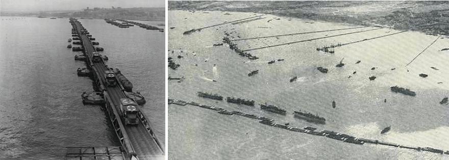
Mulberry Harbour at Arromanches, 1944 (left), Photo courtesy of Encyclopedia Britannica. Aerial view showing Mulberry Harbors at Normandy, June 1944 (right).
For the first few weeks following D-Day, the Allied forces were not able to move the front significantly inland, and danger arose that they would be boxed into Normandy until autumn and winter. This danger was enhanced when on 19 June the worst storm in nearly 40 years unexpectedly lashed Normandy (D'Este 1994).
Allied shipping between England and Normandy suffered heavy losses. About 800 ships of all sizes were beached or lost. The mobile Mulberry harbour at Omaha beach was totally destroyed and never replaced. The British Mulberry harbour at Arromanches (see picture above) was damaged, but not lost.
The storm continued for three full days. Few men or supplies could be landed in the invasion area during this period, and the 'Great Storm' in three days destroyed more vessels than the German army managed to take out during the entire campaign (D'Este 1994). The losses in material amounted to more than 140,000 tons and seriously interfered with the planned buildup of the Allied military strength in Normandy.
At the time when the storm hit Normandy, Field Marshal Rommel was attempting to assemble a powerful panzer force for a counterstroke against the Second British Army near Caen, in the western part of the invasion area. With much of the Allied air forces largely grounded during the storm, it would have been the ideal moment for Rommel to strike. However, because of the divided German command over forces in France, he was unable to do so.
Jack
Simmons (USA) very kindly suggested that the events around the storm 19-22 June 6, 1944,
would represent a fine example of how meteorological conditions affected
historical events.
1947:
Retreat of outletglaciers from Jostedalsbreen in southern Norway
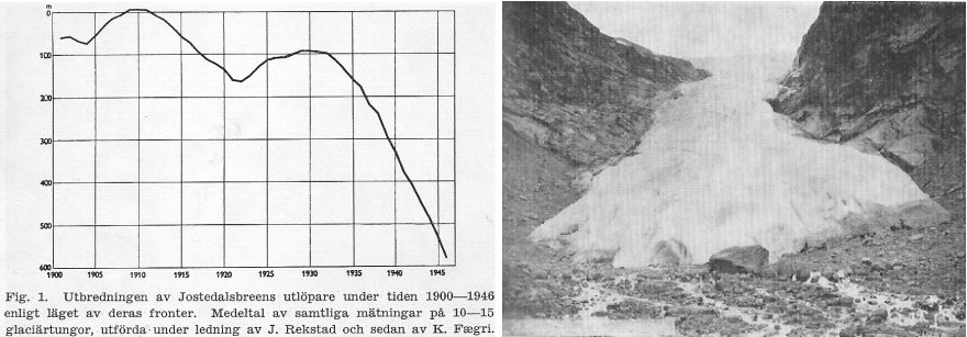
Diagram showing the average frontal retreat of 10-15 outlet glaciers from Jostedalsbreen in southern Norway (Ahlman 1947). Photo showing the terminus of the outlet glacier Mjölkevoldsbreen taken by J. Rekstad 1900 (Figure 3a in Ahlman 1947).
As documentation of the effects of the ongoing climate warming Ahlmann (1947) draws attention to the rapid glacier retreat in Norway and Sweden. He mentions that glaciers in southern Norway attained their recent maximum size during the 18th century, after witch retreat begun. A significant retreat begins around 1910, and in 1946 all monitored outlet glaciers from the big Jostedalsbreen ice cap have retreated 590 m on average. He describes the glacier retreat as almost catastrophic for some of the glaciers (Ahlnann 1947, p.292), among others the glacier Mjölkevoldsbreen (see photos above and below).
After visiting glaciers around Jostedalsbreen and in Jotunheimen, Norway, Ahlmann proceeded to inspect the glaciers in the Kebnekajse area in northern Sweden. Here the situation was found to be very much like that observed in Norway. In his own words (translated from Swedish): "Identical conditions to those observed in Jotunheimen prevailed here; ruin, sorrow and sadness about the glacier health". He also mentions that a similar situation with rapid glacier retreat applies all over Sweden.
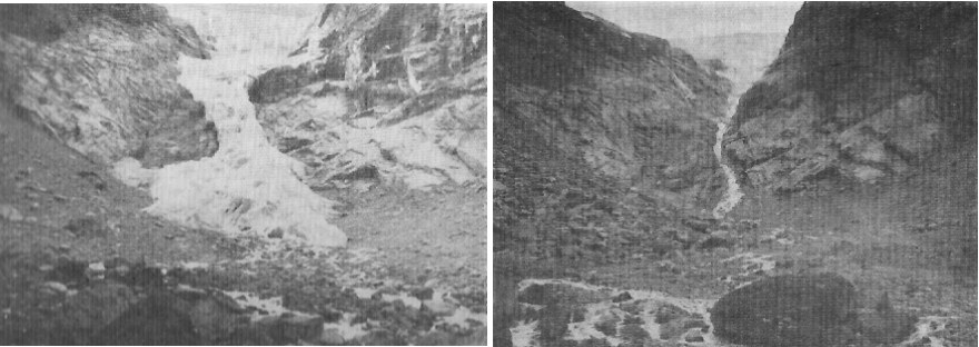
Photos showing the terminus of the outlet glacier Mjölkevoldsbreen taken by K. Fægri in August 1937 (left) and 19 July 1946 (right). Reproduced from figure 3b and 3c in Ahlmann 1947.
Click here to jump back to the list of contents.
1949:
Recent climatic fluctuations by Leo Lysgaard 

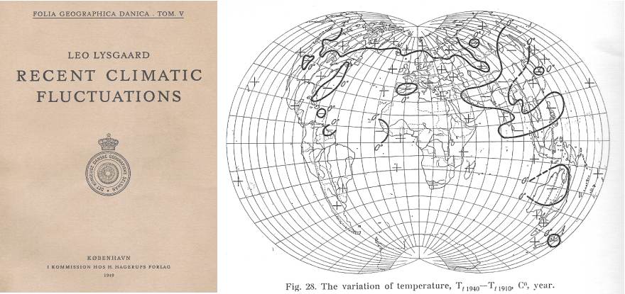
Front cover (left), and figure 28 (right) of Lysgaard 1949. The diagram shows the change of mean annual air temperature from 1910 to 1940, with highest temperature rise over the Arctic and the northern temperate zone, and less temperature increase in the southern hemisphere. Parts of Asia and Australia had experienced a temperature decrease along with the general global temperature increase. There is no data from the Antarctic.
The global temperature increase during the first part of the 20th century prompted in 1949 the publication of a major climatological thesis entitled 'Recent climatic fluctuations' by Leo Lysgaard, Danish Meteorological Institute, Copenhagen, Denmark. In the preface, Lysgaard motivates the work in the following way: "The Danish Meteorological Institute could not fail to notice the rise in temperature which took place in the Arctic regions in the twenties, and when this continued into the thirties, the present investigations were instituted to throw light, if possible, on the extent of the climatic changes or fluctuations and the cause for the same."
The publication is impressive, with a high number of tables and figures. This is before computes came into general use, so, presumably, most of the calculations must have been made by hand. Also the task of collecting meteorological data from different stations worldwide must have represented a major effort, as no global meteorological databases existed at that time. Generally, the analyses presented in the thesis are derived from calculated overlapping thirty year normals for air temperature, precipitation, pressure, gradients, direction of wind and number of sunspots, supplemented by a number of correlation coefficients between various variables.
The diagrams below show examples of the observed temperature increase winter (January) and summer (July) for a number of stations in the northern hemisphere.
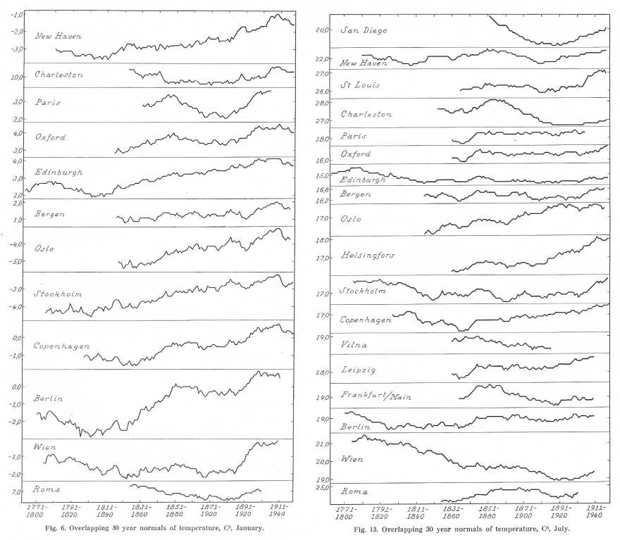
Figure 6 (left) and 13 (right) from Lysgaard 1949. Figure 6 shows the change of January temperature for a number of selected stations, while figure 13 shows the change of July temperatures. The graphs are showing overlapping values of 30-yr averages.
Lysgaard (1949) devotes a chapter (Section 5) of this thesis to discussing the cause and effect of the climatic variation. He states the following:
"According to the tables and curves, the climatic variations which have occurred during the time meteorological observations have been made are so considerable that they cannot be explained as being due to ordinary urbanization or erroneous measurements. All elements have been subjected to changes or fluctuations. In some places, especially in the Arctic regions, the January normal temperature has risen more than 3oC in recent years but the July normal has also risen more than 1oC in some places, which is of particular importance regarding the melting of the glaciers."
"The pressure and thereby the gradient and the general circulation of the atmosphere have also been subject to considerable changes or fluctuations, apart from the doldrums perhaps. The direction and velocity of the wind have both varied in the winter. The velocity has generally been increasing up to about, or just after 1930. ..... When everything else is equal, higher wind velocities should mean increasing temperatures in winter and decreasing temperatures in summer, as the air movement impedes the formation of both cold and warm surface layers of air. Air masses which flow towards colder districts will in fact bring more warmth along when the velocity increases."
Lysgaard (1949) then (p.65) list three possible ways of explaining the observed warming of the atmosphere:
-
It can, inter alia, have received more heat from the interior of the Earth.
-
It can have radiated less heat into space as a result of a change of the contents of carbon-dioxide, aqueous vapour, volcanic and electrical particles of the atmosphere.
-
It can have received more heat from the sun in consequence of a variation in solar radiation or the contents of volcanic and electric particles.
Lysgaard (1949) then proceeds (p.65): "As regards Point 1, the quantity of heat which the atmosphere receives from the interior of the earth is extremely insignificant and as far as is known, no measurements exists indicating that the rise in temperature and the increased atmospheric circulation of recent years should be due to the heat of the earth."
"As to the other points, no measurements exist either which indicate that the carbon-dioxide contents have so increased that they have importance for the hot-house effect of the atmosphere. The course of the curves seems also to show that the carbon-dioxide cannot have caused the climatic variation."
(p.66): "We will, however, keep to the causes of the present climatic fluctuations and to indications that the cause is to be found in an increase of solar radiation. One must prognosticate here that an increase of solar activity does not necessarily cause a rise in temperature over the whole earth, in any case not immediately. It is so that a variation in one weather element will inevitably cause variations in all other elements, a state of affairs which makes the whole problem so intricate and beyond computation. A temporary fluctuation of the solar radiation can thus very well produce a climatic fluctuation of considerably longer duration on the earth."
Click here to jump back to the list of contents.